Error in Mathscript (FOPDT Transfer Function)

[YukiWong]

Hi all, i am trying to write a First Order Plus Dead Time system into the mathscript, unfortunetaly i found that it appear an error (please refer to the attachements), do anyone have idea or approach to write an FOPDT Transfer function in mathscript? 

Thankyou veery much.

[Barp]

Yuki

You have to substitute the function:

plant = tf(num,den,'inputdelay',0.06)

with

Gp=set(plant,'inputdelay',0.06);

This will set the input delay for the transfer function model. The third argument for the tf command is used to set 'discrete' system with its sampling time. So, the whole script should be:

s=tf('s');

num=58;

den=0.33*s+1;

Gp =num/den;

Gp =set(plant,'inputdelay',0.06);

contr = Kp*(1/Ti*s);

sys_cl=feedback (contr*Gp,1);

hope this helps

[Barp · Accepted solution]

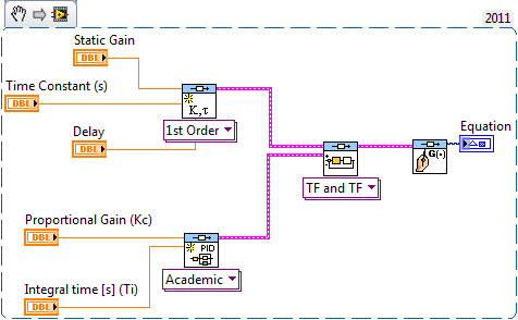
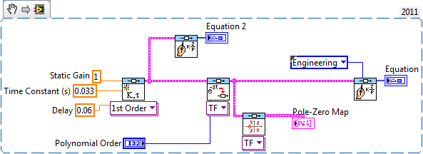
One more thing... this could be easier if you go 100% graphical...

This below is a snippet and you can just drag and drop in your LabVIEW 2011 block diagram and this will copy this code into it.

[YukiWong]

Thank you very much barp, both method work for me, but now i had face another problem.

I had try your method and design the PI controller, but the result (overshoot) is different compare to the result (overshoot) by using Matlab.

I had try to copy and paste the code from the Mathscript to the Matlab and step plot it. Consequently, the overshoot shown different value. 

I also had try to check all the value and i found that everything is ok until the last line sys_cl=feedback(Gf,1), Labview has given the answer in transfer function but Matlab has show the answer in continuous time state space model. 

The value of the transfer function : Gain = 58.46; Time constant = 0.55 and time delay = 0.06.

The value of Pi controller : Kp = 0.0784 and the Ti = 0.24. 

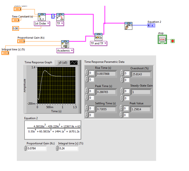
I had attach some picture which show the difference.

Am i did something wrong in the mathscript and should i do it in Labview by different way?

Thankyou very much 🙂

[YukiWong]

This is the regarding Labview file, could you please help me take a look?

Thankyou very much barp :).

[Barp]

Yuki

The problem is the delay from the First Order Model. If you look at the output error of "Unit Feedback Function", you will see a warning that says

Warning 41504 occurred at NI_CD_Model Interconnection.lvlib:cd_Feedback (TF and TF).vi

Possible reason(s):

Control Design and Simulation:  The delay information was ignored.

The main reason is that feedback function doesn't support delays. If you try to develop the model based on algebra, we can't represent the result as "exp (-D.s) *Num/Den".

To allow you to analyze such systems, you have two options:

1. Use Pade Approximation to obtain an equivalent model that of the delay and then, you can do the analysis as usual

2. Use the function "Pade" in MathScript RT to convert the model. The command line is "Gp = pade (Gp, 3)";

This should allow you to analyze the model.

[YukiWong]

thanks barp, thankyou very much, i had try out and it iss very useful for me, according to the previous graph u show me, there is a non-minimum phase behaviour occur in the response, i dont have zero on the right hand s-plane, but why the graph shown non-minimum phase behaviour? i mean it go opposite direction from the final direction. 

thankyou very much barp :).

[Barp]

Yuki

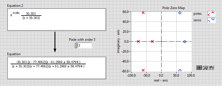
The non-minimum behavior comes from applying the pade approximation to convert the delay [exp (-0.06 s)] into a polynomial. For example, for order 3, the model has the following approximation:

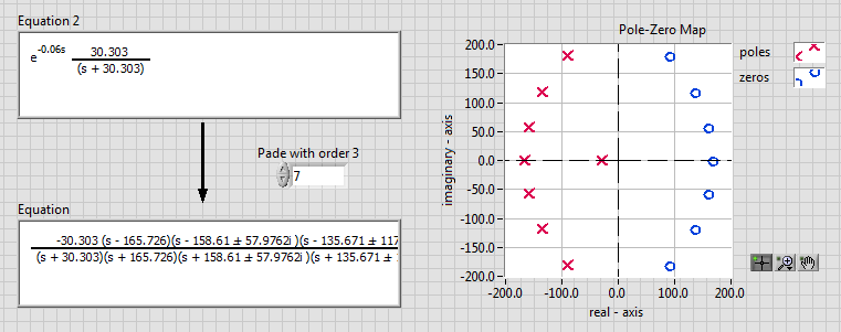
Which shows 3 zeros on the left side. If you increase this to 7, you will notice the pattern of zeros being formed on the left like this:

Here is the code related to this approximation, so you can 'play' with this code to understand.

Does it make sense?

[Barp]

Yuki

Just to be complete here. The reason you have to convert to pade approximation is because when you have a model with delay and you try to do the feedback loop operation, defined as:

Gcc = Gp*Gc/ ( 1 + Gp*Gc)

and you have a delay on Gp, you can't separated the exp (- Td*s) from the closed-loop equation and, in our toolkit, we can't use that. To overcome this problem, you can do the pade approximation we discussed above or you can try to use do nonlinear simulation. Then, you can develop the code as:

and you will see the response without the 'nonminimum phase effect'.

[Barp]

Here is the VI, to save you time.