discrete sum

[longwu2000]

Hey

Im trying to achieve a equationX_k=X_(k-1)+signal(A).  signal A is a generated signal (I tested with a sin function). I try to do it different way as shown 1 2 3 suppose to be the results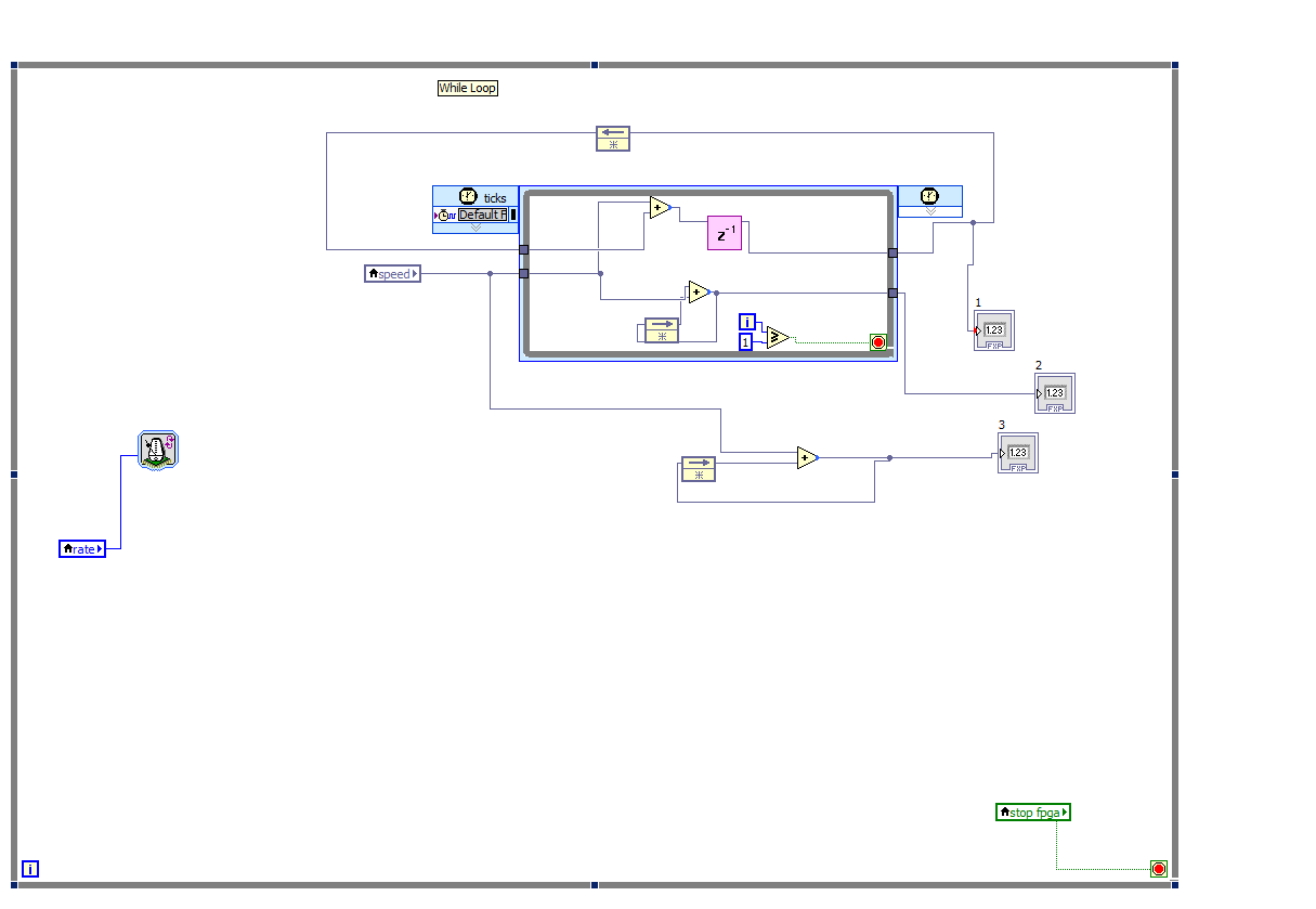

but none of the 3 is  working. I just want to know if somebody knows how to do it

Thank you

[AL3]

Hi,

at first in the FPGA I would suggest to not use the cycle counter   because it is a 32 bit data. If you want only one execution just place a constant to the exit node. If the condition is STOP IF TRUE, place a constant TRUE and it will result in a single execution.

I assume SPEED in the generated signal.

Please post the VI.

Cheers,

AL3

[longwu2000]

yes as i said the speed is just a sin wave i generateed.

i dont quit understand what you mean, i attachemnt the VI if its not much trouble would you please just change the vi to the version that you think will work

thank you

[AL3]

What you have to do is a kind of integration.

Have a look to the attached image that is related to a high performance PI controller with on-line parameter discretization. Be carefult to saturation/overflow.

[BMac]

An approach I find very productive for algorithm engineering collaborations like this is to first define the psuedocode for the math describing each of the functions, while also defining each variable and the expected behavior of the IP core. In the case that units are important to the result, it is also very important that we define the units. I recommend we all use SI (m.k.s) units whenever possible.

So... would you mind describing your intentions for the algorithm using this approach? Then we can better collaborate with you in implementing it. Let me share a couple of examples, to explain what I mean.

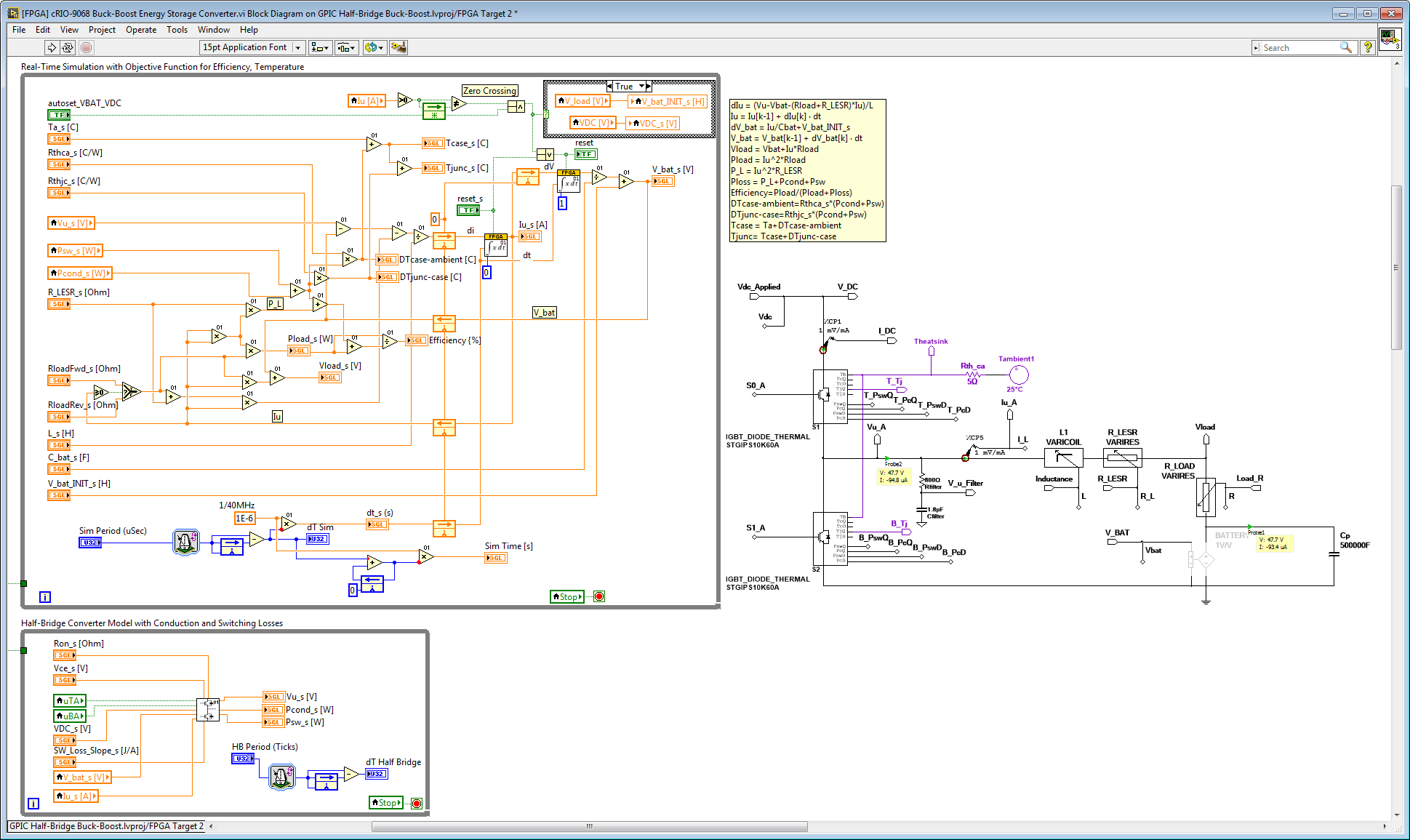
Here are some examples of Euler and Trapezoidal integration solver IP cores for LabVIEW FPGA. These are very useful for creating a real-time simulation based on any set of first order differential equations. Below I list the psuedocode for the algorithm, define the variables and expected behavior, show the LabVIEW FPGA implementation, and give directory paths to download the open source code.

[FPGA] DiscreteIntegrator RK1 Multichannel 00.vi

Description: First order Runge-Kutta 1 integration solver (Euler method)

Psuedocode: x = x[k-1] + dx · dt

Definitions & Behavior: In this implementation the input, dx (k), is assumed to be the first order derivative of x in time. dt(s) is the step size in seconds between calls to the IP core. x0 is the initial value for x(k), which is latched upon assertion of reset or in the case that the state value is NaN, Inf, or -Inf.

LabVIEW FPGA code:

IP Core Location in Power Electronics Library: C:\LabVIEW 2015\IP Cores\IP Cores - LabVIEW FPGA\HIL Solver\[FPGA] DiscreteIntegrator RK1 Multichannel 00.vi

Example Location: C:\LabVIEW 2015\GPIC\GPIC Half-Bridge Buck-Boost\Sensorless Maglev\FPGA\[FPGA] cRIO-9068 Buck-Boost Energy Storage Converter.vi

Example Psuedocode and Screenshot:

Description: This is a real-time simulator for a half-bridge buck-boost energy storage converter that runs efficiently on small FPGA targets such as the sbRIO-9606 GPIC. The electrical model is derived from Kirchoff's Voltage Law (KVL) and Kirchoff's Current Law (KCL) for the half-bridge circuit. The energy storage battery is modeled as a large capacitance (C_bat = Reserve_Capacity_Minutes*25*60/Nominal_Voltage, and Amp_hours = Reserve_Capacity_Minutes*25/60) with charge and discharge resistances. The simulator includes energy efficiency calculations, where charging the battery and the resistive losses in the battery are considered useful work (Pload). On the other hand, losses in the converter (switching and conduction losses) and series resistance losses in the buck-boost series inductor are considered waste power (Ploss). The simulator also includes a transient thermal model that calculates the IGBT junction temperature and case temperature. This model can be used as an observer for active junction temperature regulation by replacing the calculated phase current with measured phase current and regulating the switching frequency and DCLink voltage to achieve the desired junction temperature. Note that Tjunc and Tcase in this model represent the values that would occur in the future (steady-state) if the existing circuit conditions (i.e. current, switching frequency, DC link voltage, etc.) were held steady. Therefore the Tjunc and Tcase values are actually zero-delay observers, where the transient delays of the thermal network are intentionally excluded (at this stage of the model) to facilitate active junction temperature regulation. By using the zero-delay observer values, the junction temperature can be more tightly controlled since the control system is able to anticipate and pre-emptively adjust to regulate the temperature without time delays. Integral action is required on the PID controller for use with the zero delay observer value.

dIu = (Vu-Vbat-(Rload+R_LESR)*Iu)/L

Iu = Iu[k-1] + dIu · dt

dV_bat = Iu/Cbat+V_bat_INIT_s

V_bat = V_bat[k-1] + dV_bat · dt

Vload = Vbat+Iu*Rload

Pload = C*Vbat*dV_bat+Iu^2*Rload

P_L = Iu^2*R_LESR

Ploss = P_L+Pcond+Psw

Efficiency=Pload/(Pload+Ploss)

DTcase-ambient=Rthca_s*(Pcond+Psw)

DTjunc-case=Rthjc_s*(Pcond+Psw)

Tcase = Ta+DTcase-ambient

Tjunc= Tcase+DTjunc-case

In another example (C:\LabVIEW 2015\GPIC\GPIC Half-Bridge Buck-Boost\Sensorless Maglev\FPGA\[FPGA] NI GPIC Buck-Boost Energy Storage Converter.vi), the transient thermal behavior of the junction and case temperatures with delays is modeled using a 9th order Cauer thermal impedance model implemented using first order low pass filters. (Please check my implementation.) These simulated temperature values, Tjunc_s_f and Tcase_s_f , can be expected to match physical measurements. 

Here is how the junction temperature regulation is incorporated in the PID control loop. The “instantaneous steady state” junction temperature is used for regulation (a.k.a. zero delay observer). In this case I’m adjusting switching frequency only within a determined range (which is set in the PID Channel Config.).

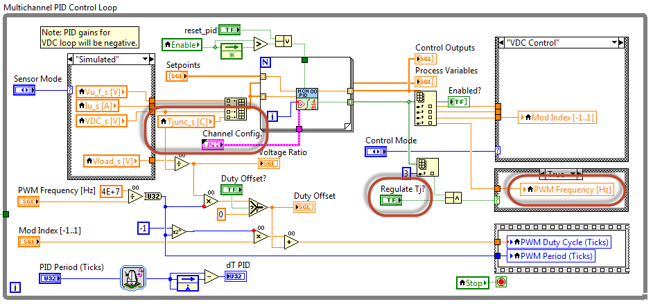
The manufacturer datasheet information (equivalent transient thermal network) is used to construct the low pass filter coefficients for the LabVIEW FPGA transient thermal impedance model. In the case that the vendor does not provide R, C values for an equivalent Foster or Cauer network, note that the Semikron SEMISEL (desktop) tool can facilitate finding the equivalent R,C values given transient thermal impedance chart data.

[FPGA] DiscreteIntegrator Trapezoidal Multichannel 02.vi

Description: Integration solver based on the Trapezoidal rule. Compared to the Euler method, this often provides more accurate integration when using larger timesteps and for signals with harmonics.

Psuedocode: x = x[k-1] + 0.5 · (dx+dx[k-1]) · dt

Definitions & Behavior: In this implementation the input, dx (k), is assumed to be the first order derivative of x in time. dt(s) is the step size in seconds between calls to the IP core. x0 is the initial value for x(k), which is latched upon assertion of reset or in the case that the state value is NaN. max is the maximum allowed value for x(k). In the case that x(k) is being coerced to the max value, max limited? is true. min is the maximum allowed value for x(k). In the case that x(k) is being coerced to the min value, max limited? is true.

LabVIEW FPGA code:

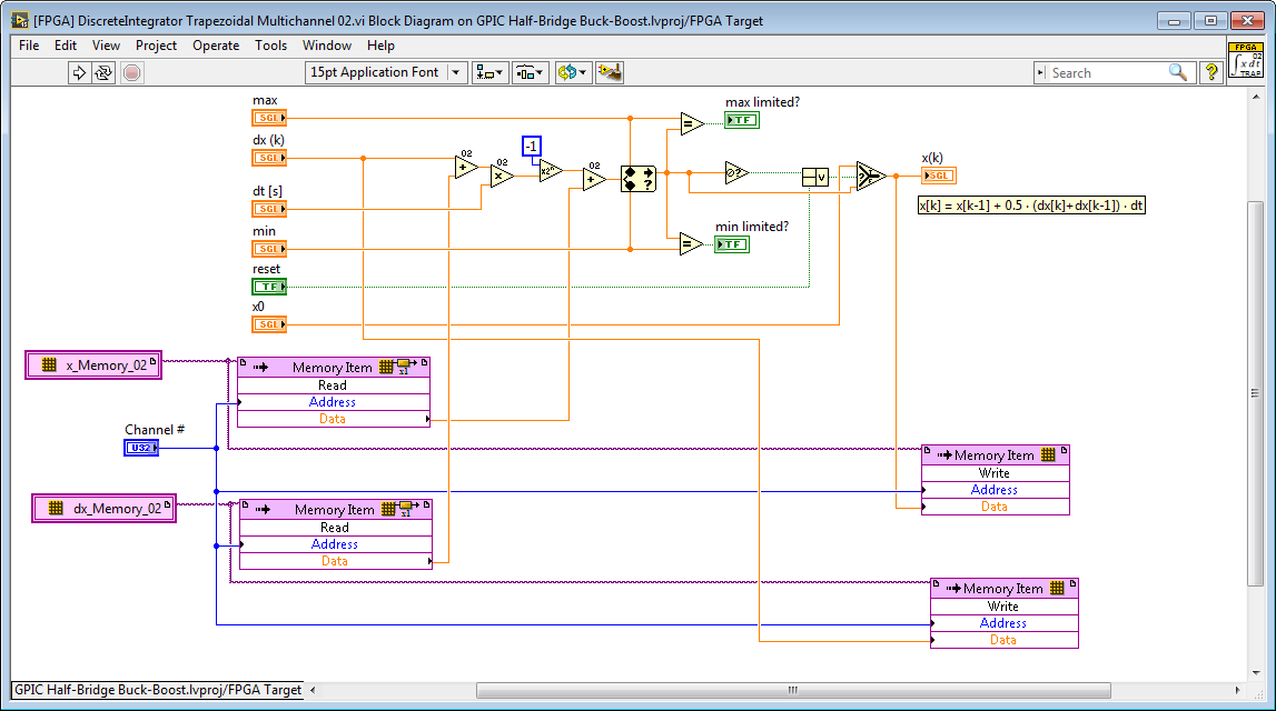
IP Core Location in Power Electronics Library: C:\LabVIEW 2015\IP Cores\IP Cores - LabVIEW FPGA\HIL Solver\Polymorphic subVIs\[FPGA] DiscreteIntegrator Trapezoidal Multichannel 02.vi

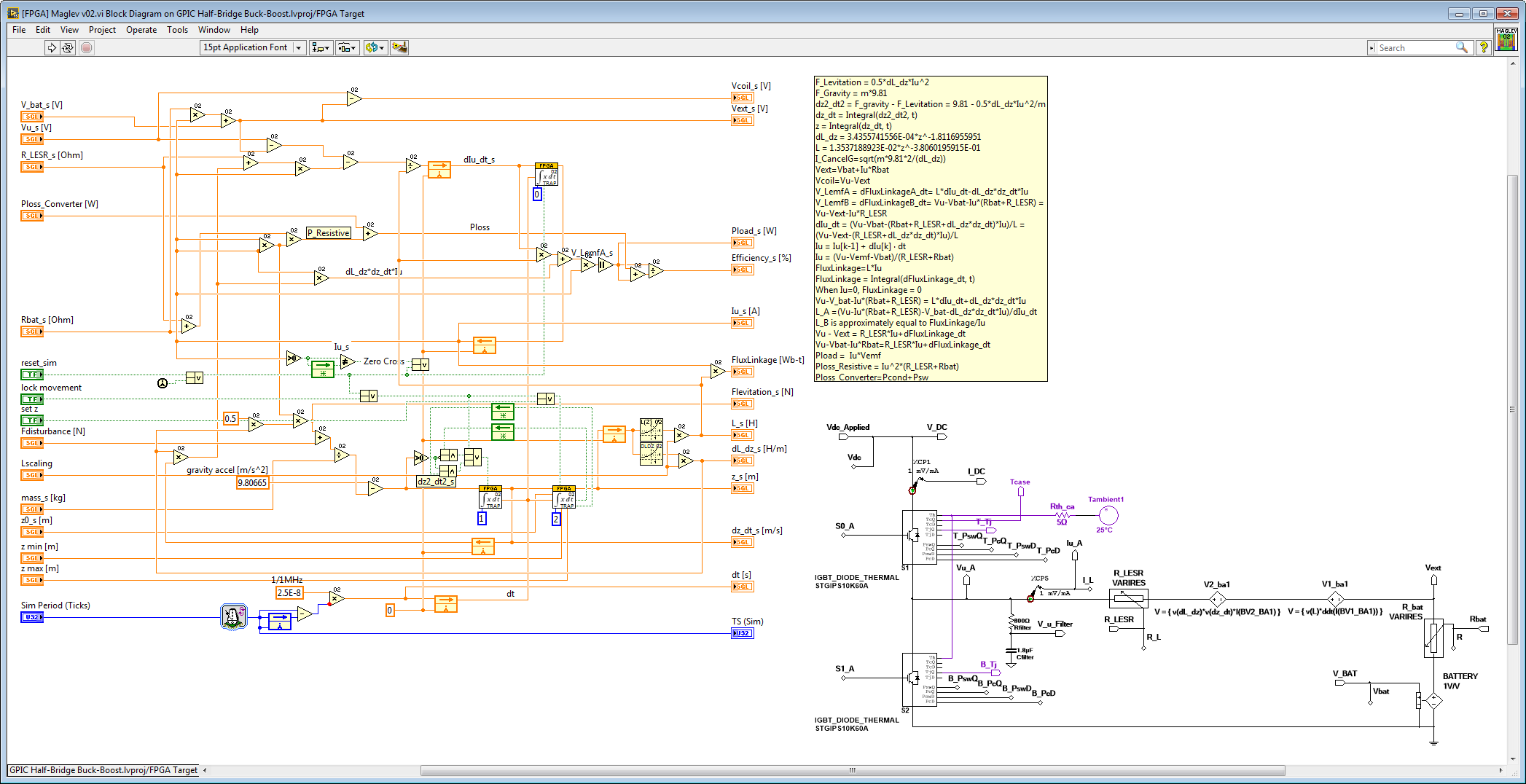
Example Location: C:\LabVIEW 2015\IP Cores\IP Cores - LabVIEW FPGA\HIL Solver\[FPGA] Maglev v02.vi

Example Psuedocode and Screenshot:

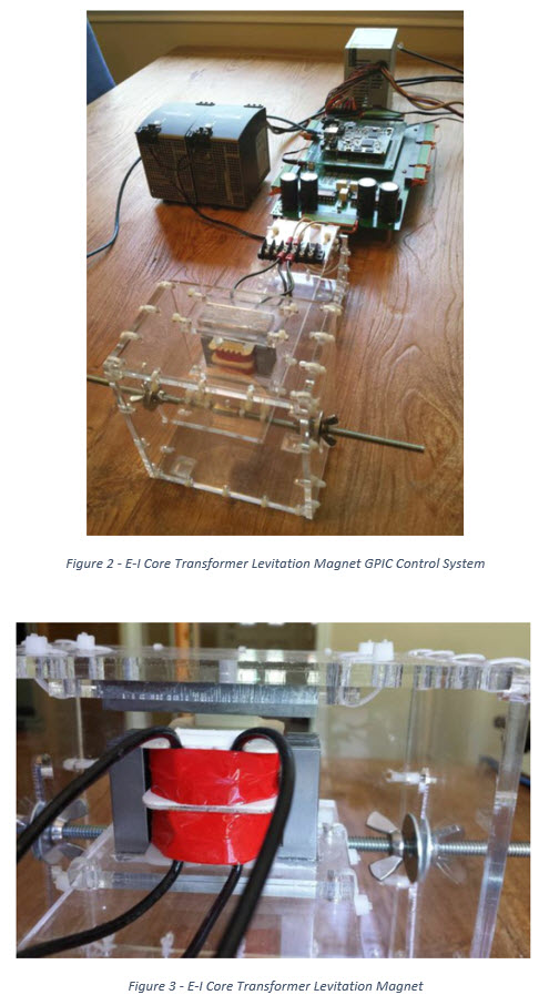
Description: This is a real-time simulator for a non-linear E-I transformer core magnetic levitation system including energy efficiency calculations, where the current in the moving E core windings (rotor/translator) is controlled by an IGBT half-bridge. It is an electromechanical simulation, assuming one-degree of freedom (vertical z-axis) levitation of the vehicle. This type of maglev can easily be constructed by purchasing a standard low cost E-I core transformer, dissassembling it to remove the I core laminations (using razor blade), and then re-stacking and attaching the I core laminations to the stationary track as the non-moving part (stator/track)- see photos below. Non-linear equations for inductance as a function of z-axis position, L(z), and z-axis partial derivative of inductance with respect to z-axis position, dL_dz(z) are encoded as look up tables with linear interpolation. The Integral(dx, t) notation refers to the trapezoidal integrator core described above. This runs efficiently in floating point, along with the control and analysis IP, on the Spartan-6 LX45T FPGA of the sbRIO-9606 GPIC.

Psuedocode:

F_Levitation = 0.5*dL_dz*Iu^2

F_Gravity = m*9.81

dz2_dt2 = F_gravity - F_Levitation = 9.81 - 0.5*dL_dz*Iu^2/m

dz_dt = Integral(dz2_dt2, t)

z = Integral(dz_dt, t)

dL_dz = 3.4355741556E-04*z^-1.8116955951

L = 1.3537188923E-02*z^-3.8060195915E-01

I_CancelG=sqrt(m*9.81*2/(dL_dz))

Vext=Vbat+Iu*Rbat

Vcoil=Vu-Vext

V_LemfA = dFluxLinkageA_dt= L*dIu_dt-dL_dz*dz_dt*Iu

V_LemfB = dFluxLinkageB_dt= Vu-Vbat-Iu*(Rbat+R_LESR) = Vu-Vext-Iu*R_LESR

dIu_dt = (Vu-Vbat-(Rbat+R_LESR+dL_dz*dz_dt)*Iu)/L =

(Vu-Vext-(R_LESR+dL_dz*dz_dt)*Iu)/L

Iu = Iu[k-1] + dIu · dt

Iu = (Vu-Vemf-Vbat)/(R_LESR+Rbat)

FluxLinkage=L*Iu

FluxLinkage = Integral(dFluxLinkage_dt, t)

When Iu=0, FluxLinkage = 0

Vu-V_bat-Iu*(Rbat+R_LESR) = L*dIu_dt+dL_dz*dz_dt*Iu

L_A =(Vu-Iu*(Rbat+R_LESR)-V_bat-dL_dz*dz_dt*Iu)/dIu_dt

L_B is approximately equal to FluxLinkage/Iu

Vu - Vext = R_LESR*Iu+dFluxLinkage_dt

Vu-Vbat-Iu*Rbat=R_LESR*Iu+dFluxLinkage_dt

Pload =  Iu*Vemf

Ploss_Resistive = Iu^2*(R_LESR+Rbat)

Ploss_Converter=Pcond+Psw

Photos:

Note that the required inductive air gap proximity sensor is not shown in the photos below.

Additional Notes:

1. I've written these IP cores to be multi-channel, so rather than using feedback nodes to store state (history) values I use FPGA RAM, which is addressed using the Channel #. In this way, the state values for each channel are held in unique memory locations.

2. For the math operators in each IP core (add, subtract, multiply, etc.), I'm also using non-reentrant subVIs which are therefore shared by all callers. The top level multi-channel IP core is also set to be non-reentrant (File>VI Properties>Execution).

[longwu2000]

Thank you for the reply. I think my problem is a Euler kind of problem. What im trying to do is a speed observer. Which X_k=X_(k-1)+signal(A). X_k is the current speed, X_k-1 is the last iteration speed and the signal(A) is the acceleration times the dt. The initial condition of speed is 0 and acceleration is genrated by using other states of a motor.

I will give it a try using the Euler example you gave.

And Im currently out of lab this winter, will get back in Jan hopefully we can still continue this discussion when I get back to the lab

thank you