- Subscribe to RSS Feed
- Mark Topic as New
- Mark Topic as Read
- Float this Topic for Current User
- Bookmark
- Subscribe
- Mute
- Printer Friendly Page
Practical Nonlinear Fitting
03-05-2011 12:25 PM
- Mark as New
- Bookmark
- Subscribe
- Mute
- Subscribe to RSS Feed
- Permalink
- Report to a Moderator
Summary:
Fitting of experimental data to a nonlinear model is a very common task in science. It allows the parameterization of potentially huge amounts of data based on a given mathematical model.
A simple example would be an exponentially decaying curve: We start out with thousands of potentially meaningless points and end up with an (1) amplitude, (2) decay constant, (3) offset (and an estimate of the noise in the data). These three parameters can fully describe the data in terms of a few physically meaningful numbers if the model is correct.
It is obvious that a successful fit requires a proper choice of a model. If we would try to fit the same exponential data to a Gaussian line shape or a high order polynomial, we might get an equally good fit, but the resulting parameters would be completely meaningless.
With LabVIEW 8.0, nonlinear least square fitting has become flexible, simple and powerful. (Pre-8.0, you typically needed to roll your own, because the stock LabVIEW fitting tools were basically unusable). With the current design (model reference, "Data" variant input, etc.) anything (anything!!!) is now possible and I have posted numerous specific examples in the LabVIEW forum over the years dealing with 1D and 2D data. An example of what can be done is my fitting program for multicomponent EPR spectra. Here the model contains up to ~150 parameters and any subset can be selected to be fit, with the remaining parameters held fixed based on prior knowledge.
The example attached below will serve as guidelines for beginners on how to implement several useful basic techniques that will make nonlinear fitting flexible and scalable. For the first round I will introduce a simple example showing a way to:
- Make the model scalable for a variable number of components so we don't need to rewrite it every time the number of components changes.
- Allow a run time selection of a subset of parameters to be fit. This way we need to write the model only once, and not a seperate version for each combination of parameters.
- ...
In later rounds, I might expand to 2D data, global fitting, ways to handle parameter names, allow real-time monitoring and interruption of the fitting, show how to calculate, format and interpret the correlation matrix, estimate parameter errors, and other useful techniques that anybody in this field should be familiar with.
Over the years, I have posted countless nonlinear fitting examples of various complexity in the LabVIEW forum. My contribution here will be new, general, scalable, and of common interest.
Function:
This collection of VIs introduce the concept of nonliner fitting
Example 1:
This is the most basic example distillied to the essentials for simplicity.
It fits a simple exponential decay with three parameters
1. offset
2. amplitude
3. decay constant
Y(t)=Amplitude * exp(-t/decay constant) + offset
Example 2:
Once you understand the simple fit, we add two features to make the code more useful:
scaleable, so it automatically adapts to a multiexponential fit
flexible, so we can select a subset of parameters to be fitted while holding some constant
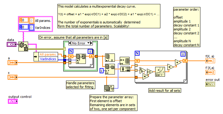
Y(t) = offset + a1 * exp(-t/DC1) + a2 * exp(-t/DC2) + a3 * exp(-t/DC3) + ...
with the number of terms automatically adjusting based on the number of parameters.
Example 3:
In example 2, we made the model scalable. Now we utilize that feature to fit a double-exponential decay.
Y(t) = offset + a1 * exp(-t/DC1) + a2 * exp(-t/DC2)
Now that the model is a bit more complicated, we might run into issues with correlated parameters. In such a case a change in one parameter can be more or less compensated by a change in another parameter. For example if DC1 and DC2 are very similar, an increase in a1 can be nearly compensated by an opposite change in a2. To identify correlations, we can calculate the correlation matrix from the covariance matrix. Values near 1 or -1 indicate strong correlation. To obtain a meaningful fit, only one of the correlated parameters should be used for fitting, while the others should be held constant and a reasonable value.
Exercise: See how the correlation changes. (1) using the default parameters, (2) making both TCs the same, (3) making TCs very long (e.g. 1 and 2). If the TCs are long compared to the sampled time, the curve is nearly linear and everything becomes correlated. THe situation improves for example if we know the offset and keep it fixed.
Steps to execute code:
- Open the project.
- Open the simple fit
- Study the code and the model. It is intentionally simple (no event structure, and other constructs)
- run it according to the instruction on the front panel
- Once you understand the code ...
- Open the Advance Fit
- Study the code and the model. Compare the additional code to increase functionality
Screenshots:
Main Front Panel:
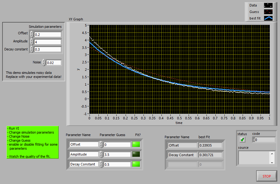
This is the advanced panel. The amplitude was excluded from fitting, thus the poor quality.
VI Snippet:
No snippet, just images. A snippet cannot duplicate the strictly typed connector pattern needed for the fitting routines.
Simple model

Advanced model
An image of the code that convert the covariance matrix to the formatted correlation matrix.

VI attached below
Main version is in LabVIEW 2010
(A LabVIEW 8.2 version is also attached).
03-06-2011 05:34 PM
- Mark as New
- Bookmark
- Subscribe
- Mute
- Subscribe to RSS Feed
- Permalink
- Report to a Moderator
I'm interested to see what you end up posting. I have a feeling it will make my brain hurt but I will learn a lot 
03-07-2011 11:28 AM
- Mark as New
- Bookmark
- Subscribe
- Mute
- Subscribe to RSS Feed
- Permalink
- Report to a Moderator
Nice work! I'm already following your group so I can learn more.
02-20-2013 05:38 AM
- Mark as New
- Bookmark
- Subscribe
- Mute
- Subscribe to RSS Feed
- Permalink
- Report to a Moderator
Hi Altenbach, I have found this along with many of your posts on non-linear LM fitting really useful for developing efficient fitting code for the lab. In a number of posts where you give examples of improvements to the core LV implementation, for example in optimising the workings of the ABX function (http://forums.ni.com/t5/LabVIEW/Heavy-bug-in-quot-exponential-fit-quot/td-p/2249096) and giving your own fitting code in the 2D surface fit (http://forums.ni.com/t5/LabVIEW/How-do-I-fit-a-curve-with-two-independant-variables/m-p/138027). Just wondered if you have a definite "best" version of your LM code, and if so whether you could point me in its direction if already included in a forum post, or if you actually optimise choices for each application (for example whether parrallelised loops or not?)
02-20-2013 03:37 PM
- Mark as New
- Bookmark
- Subscribe
- Mute
- Subscribe to RSS Feed
- Permalink
- Report to a Moderator
Jim brought up a few good points here.
The rewrite of ABX is a relatively unimportant issue and only increases performance, which is usually not a limiting factor.
More useful is the ability to modify the lambda scaling (starting lambda, sclae up factor, scale down factor) and the update mode. For my own use I modified the stock VIs to allow setting these parameters. I played a lot with various of the NIST datasets, and some of the more difficult are just plain silly and seem to be designed to not converge well from certain starting points. For real-world problems and resonable starting parameters, these issues are typically not a problem and the lambda settings can be optimized for better initial convergence. For my own fitting, I see a dramatic improvements under all conditions when starting with a smaller lambda. With the stock lambda, the SSE lingers for quite a few iterations before it drops like a rock to the optimum. With a smaller starting lambda, the initial drop happens right away. (If the lambda is too small, the drop is fast, but then it often goes back up chaotically, before settling). Having Lambda exposed also gives you some other algorithms for free. For example, you can set the value to zero to do a pure conjugate gradient fit.
Please ignore the old ABX stuff. This was all written before LabVIEW 8.0, which received a major overhaul of all the fitting VIs. Pre 8.0, the stock Levenberg Marquard fitting was nearly useless because you could not even change the model without rewriting the entire set of VIs. Back then, I wrote my own to be able to call the model by reference. (Me and Don Wagner also helped Dave Thomson back in the LabVIEW 6.0 days to improve the VIs)
02-20-2013 06:02 PM
- Mark as New
- Bookmark
- Subscribe
- Mute
- Subscribe to RSS Feed
- Permalink
- Report to a Moderator
Thanks for taking the time to reply - I will take out the old routines and just try playing around with lambda as suggested!
07-28-2020 01:57 PM - edited 07-28-2020 01:59 PM
- Mark as New
- Bookmark
- Subscribe
- Mute
- Subscribe to RSS Feed
- Permalink
- Report to a Moderator
Wow, this is a really old topic (2011!).
Yet, I am very happy with it.
Thanks a lot.
Curve fitting is something I need from time to time, but modelling in LabVIEW is not so easy for me. Could also be a lack of fundamental math knowledge (not used to think in matrices, for instance). In that respect it is much easier to use the solver in excel, just point to cells and force them to a desirable value. You can easily restrict parameters there. However, in another sense it is also less powerful, and too often it will not find a solution. Needs clever thinking too 😉.
Just this simple exponential decay example is exactly what I need and works like a charm, and really fast! (I started with a brute force method, which of course takes much, much longer).
A bit disappointing the examples presented here do not come as shipping examples.
As a side note: I noticed the 'Re/Im to complex'-primitives as a means to compose the formatting for the X-Y Graph. Really interesting. However, does it have an advantage over the 'good old' bundle as suggested in the context help?
07-28-2020 02:23 PM
- Mark as New
- Bookmark
- Subscribe
- Mute
- Subscribe to RSS Feed
- Permalink
- Report to a Moderator
Ah, and even more possibilities, following example 2. Especially the ability to choose whether you would like to fit a parameter or not.
This corner of LabVIEW is a grey blurr to me 😥, but at least I know how to use the bits that others have disclosed to me.
Thanks again!
In my mind I keep clicking the kudo button 😆
08-09-2020 12:02 PM
- Mark as New
- Bookmark
- Subscribe
- Mute
- Subscribe to RSS Feed
- Permalink
- Report to a Moderator
Diving a little bit further into this Nonlinear Fitting, I found it far less complicated than I thought. Even if you are not that experienced w.r.t. fitting. Of course, you do need to know what your data stands for and how it can be modeled. But implementing it, once you have Altenbachs examples, is not that difficult. I even successfully managed to implement a one-dimensional thermal node model within MODEL.vi, that needs iteration until a stop criterion is met. I first struggled a little bit with the idea that my model does not contain a single equation, but that's not a problem at all. As long as you have some that produces a single output on your input y=f(x), all is fine. In my case, it is a temperature measured along a single cooling fin in a vacuum (so radiation is the only means of thermal heat exchange). The model expects distance, and gives you temperature.
Because my MODEL.vi itself contains an iterating loop, you have to keep calculations as simple as possible within that loop (weed out everything that can be done outside that loop). Otherwise it may take a long time until a solution is found. I found out, for instance, that inlining a subvi within that iterating loop within MODEL.vi, helped to slash iteration time by a factor two.
06-13-2024 09:25 AM
- Mark as New
- Bookmark
- Subscribe
- Mute
- Subscribe to RSS Feed
- Permalink
- Report to a Moderator
Dear Altenbach,
I am trying to fit fluorescence signals that I measure on plant leaves in time. A graph is shown below that shows the kind of data that is obtained. As far as I can tell, it is an exponential increase, with offset, that starts after some delay. Would it be posible to use your vi, to fit these data? I do have some experience with Labview, but I have a hard time to understand the block diagrams of your vi's. Can you explain me how to feed an two dimensional array into the vi's that you provided?

