Demodulate and Listen to FM Radio with LabVIEW Communications and NI USRP

[C-Dav]

Overview

This example uses the USRP as a spectrum analyzer to both find local FM radio stations and listen to their live broadcast(s).

Description

This example utilizes the following scheme to perform FM demodulation for audio playback: 

1. The phase of the incoming signal is extracted using the Arctangent Method
2. Then, the phase is unwraped to remove discontinuities left by the phase extraction
3. The extracted and unwrapped phase is then differentiated
4. and finally the signal is resampled to a rate supported by a PC sound card

Steps to Implement or Execute Code:

Find an FM Radio Station

Using USRP as a Spectrum Analyzer

1.  Open the document: Find Radio Station.gvi

2.  Verify the correct IP Address of your USRP is set under device names (typically 192.168.10.2)

3.  Configure the remaining Front Panel parameters as follows:

Parameter	Value
Device names	192.168.10.2 (typically)
IQ Rate	10M
Carrier Frequency	93M
Gain (dB)	0
Active Antenna	RX1
Number of Samples	20k
Timeout	10

NOTE: Capitalization is important when entering parameters like IQ Rate and Carrier Frequency. Capital M is interpreted by LabVIEW as "Mega-" while lower case m is interpreted as "-milli."

4.  Run the VI (Note: if it errors try and decreasing the number of samples to 10,000)

5.  Note the various peaks that should be visible in the resulting Frequency Plot -- this will vary depending on the physical 6.  location where this example is performed and what FM stations are available.  Remember that 0 on the graph represents 7.  the carrier frequency specified in step 3.  An example plot os provided in Figure 1.

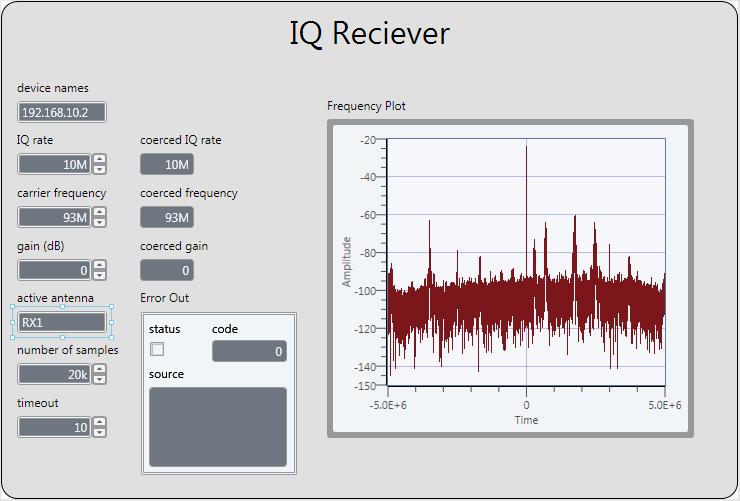
Figure 1: Frequency Plot of our region

8.  If you zoom in to a particular area (peak) of interest, you may also notice that the bandwidth of the radio station is +/- 100kHz (a total of 200kHz).

NOTE: a simple way to explore the data in LabVIEW Communications is to right click on the indication (in this example, Frequency Plot) and select Capture Data.  You can then double-click the captured data item in the Data pane on the left of the workspace to open the data view.  In this view, you can effortlessly browse the captured data set, zooming in to areas of interest and in this case identifying a particular radio station's center frequency and bandwidth.

Troubleshooting:

• If you're unable to find a station, try boosting the gain:
  • Try gain settings of 10, 25, and 30
• If you're still unable to find stations:
  • You may not have good enough reception to capture a local station.  If you aren't able to identify a radio station, playback will not be possible.  You may want to stop the demo here and check out the demo video.

Tune to a Specific FM Radio Station

1.  Once you have observed the spectrum and selected a particular station's center frequency, you can adjust the parameters of the Find Radio Stations VI to observe that station more closely.

2.  Adjust the Carrier Frequency and Bandwidth inputs to whatever you determined in the last section (we'll be using 93.7 MHz and 200 kHz, respectively)

3.  Run the VI once again, and observe the resulting Frequency Plot, similar to the one in Figure 2.

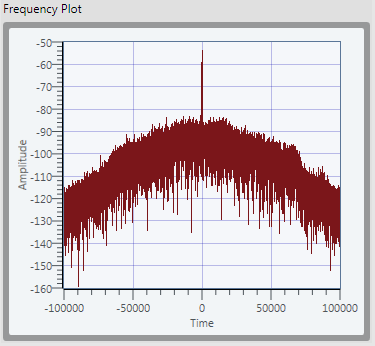
Figure 2: Frequency Plot of our tuned spectrum analysis

Listen to Live FM Radio

Now that a station has been identified, we will tune to that station and create an audio output of the live broadcast through our computer's speakers.

1. Open Main Demodulate.gvi
2. Place an MT Demodulate FM node on the diagram to the right of the niUSRP Fetch Rx Data node.
3. Place a Waveform Properties node to the right of the MT Demodulate FM node.
4. Change the carrier frequency to that of the radio station you found in the previous section
   • For example, if the center frequency is 94.7M and the station appears at -1M, set the new radio staion frequency to 93.7M
5. Decrease the IQ rate to 200kHz

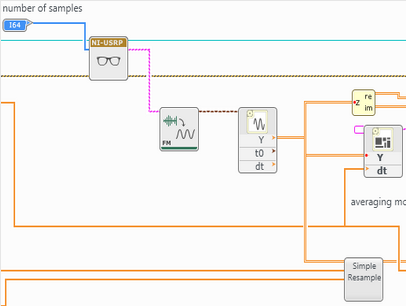
Figure 3: Final Block Diagram configuration should look like this

1. Press Ctrl+E to switch to the Front Panel of the VI.
   

2. Run the VI and listen to output.

3. You’ve now demodulated broadcast FM radio using the mathematical approach

Troubleshooting:

1. Hearing distortion?
   • Distortion can be caused by applying too little or too much gain! Try increasing the gain or decreasing the gain methodically.  Use the first part of this demo, the spectrum analyzer, to troubleshoot.
2. Hearing breaks in the audio?
   • The sound VI’s are less than ideal.  Try decreasing the number of samples to a very small number like 10,000.  Unfortunately, some PC sound cards just don’t work well.  Performace will vary case by case.

Requirements

Software

• LabVIEW Communications System Design Software or Suite 1.0
• Radio station reception (not a good demo for the basement, use the video)

Hardware

• USRP-2920, USRP-2930, USRP-2940, or USRP-2950 (most radio stations fall between 88 MHz and 108 MHz)
• Ideally an FM antenna, but any small wire may work

Additional Images or Video

LabVIEW 2014 version of this example is available here.

Click Here to discuss this and other examples on the LabVIEW Communications Discussion Forums.