Community Browser
-
NI Community
- Welcome & Announcements
-
Discussion Forums
- Most Active Software Boards
- Most Active Hardware Boards
-
Additional NI Product Boards
- Academic Hardware Products (myDAQ, myRIO)
- Automotive and Embedded Networks
- DAQExpress
- DASYLab
- Digital Multimeters (DMMs) and Precision DC Sources
- Driver Development Kit (DDK)
- Dynamic Signal Acquisition
- FOUNDATION Fieldbus
- High-Speed Digitizers
- Industrial Communications
- IF-RIO
- LabVIEW Communications System Design Suite
- LabVIEW Electrical Power Toolkit
- LabVIEW Embedded
- LabVIEW for LEGO MINDSTORMS and LabVIEW for Education
- LabVIEW MathScript RT Module
- LabVIEW Web UI Builder and Data Dashboard
- MATRIXx
- Hobbyist Toolkit
- Measure
- NI Package Manager (NIPM)
- Phase Matrix Products
- RF Measurement Devices
- SignalExpress
- Signal Generators
- Switch Hardware and Software
- USRP Software Radio
- NI ELVIS
- VeriStand
- NI VideoMASTER and NI AudioMASTER
- VirtualBench
- Volume License Manager and Automated Software Installation
- VXI and VME
- Wireless Sensor Networks
- PAtools
- Special Interest Boards
- Community Documents
- Example Programs
-
User Groups
-
Local User Groups (LUGs)
- Denver - ALARM
- Bay Area LabVIEW User Group
- British Columbia LabVIEW User Group Community
- Chicago LabVIEW User Group
- Egypt NI Chapter
- GUNS
- Houston Area LabVIEW Community
- LabVIEW - University of Applied Sciences Esslingen
- [IDLE] LabVIEW User Group Stuttgart
- LUGG - LabVIEW User Group at Goddard
- LUGNuts: LabVIEW User Group for Connecticut
- Madison LabVIEW User Group Community
- Mass Compilers
- Melbourne LabVIEW User Group
- Midlands LabVIEW User Group
- Milwaukee LabVIEW Community
- Minneapolis LabVIEW User Group
- CSLUG - Central South LabVIEW User Group (UK)
- Nebraska LabVIEW User Community
- New Zealand LabVIEW Users Group
- NI UK and Ireland LabVIEW User Group
- NOCLUG
- Orange County LabVIEW Community
- Ottawa and Montréal LabVIEW User Community
- Washington Community Group
- Phoenix LabVIEW User Group (PLUG)
- Politechnika Warszawska
- PolŚl
- Rutherford Appleton Laboratory
- Sacramento Area LabVIEW User Group
- San Diego LabVIEW Users
- Sheffield LabVIEW User Group
- South East Michigan LabVIEW User Group
- Stockholm LabVIEW User Group (STHLUG)
- Southern Ontario LabVIEW User Group Community
- SoWLUG (UK)
- Space Coast Area LabVIEW User Group
- Sydney User Group
- Top of Utah LabVIEW User Group
- Utahns Using TestStand (UUT)
- UVLabVIEW
- Western NY LabVIEW User Group
- Western PA LabVIEW Users
- Orlando LabVIEW User Group
- Aberdeen LabVIEW User Group (Maryland)
- Gainesville LabVIEW User Group
- LabVIEW Team Indonesia
- Ireland LabVIEW User Group Community
- Louisville KY LabView User Group
- NWUKLUG
- LVUG Hamburg
- LabVIEW User Group Munich
- LUGE - Rhône-Alpes et plus loin
- London LabVIEW User Group
- VeriStand: Romania Team
- DutLUG - Dutch LabVIEW Usergroup
- WaFL - Salt Lake City Utah USA
- Highland Rim LabVIEW User Group
- NOBLUG - North Of Britain LabVIEW User Group
- North Oakland County LabVIEW User Group
- Oregon LabVIEW User Group
- WUELUG - Würzburg LabVIEW User Group (DE)
- LabVIEW User Group Euregio
- Silesian LabVIEW User Group (PL)
- Indian LabVIEW Users Group (IndLUG)
- West Sweden LabVIEW User Group
- Advanced LabVIEW User Group Denmark
- Automated T&M User Group Denmark
- UKTAG – UK Test Automation Group
- Budapest LabVIEW User Group (BudLUG)
- South Sweden LabVIEW User Group
- GLA Summit - For all LabVIEW and TestStand Enthusiasts!
- Bangalore LUG (BlrLUG)
- Chennai LUG (CHNLUG)
- Hyderabad LUG (HydLUG)
- LUG of Kolkata & East India (EastLUG)
- Delhi NCR (NCRLUG)
- Montreal/Quebec LabVIEW User Group Community - QLUG
- Zero Mile LUG of Nagpur (ZMLUG)
- LabVIEW LATAM
- LabVIEW User Group Berlin
- WPAFB NI User Group
- Rhein-Main Local User Group (RMLUG)
- Huntsville Alabama LabVIEW User Group
- LabVIEW Vietnam
- [IDLE] ALVIN
- [IDLE] Barcelona LabVIEW Academic User Group
- [IDLE] The Boston LabVIEW User Group Community
- [IDLE] Brazil User Group
- [IDLE] Calgary LabVIEW User Group Community
- [IDLE] CLUG : Cambridge LabVIEW User Group (UK)
- [IDLE] CLUG - Charlotte LabVIEW User Group
- [IDLE] Central Texas LabVIEW User Community
- [IDLE] Cowtown G Slingers - Fort Worth LabVIEW User Group
- [IDLE] Dallas User Group Community
- [IDLE] Grupo de Usuarios LabVIEW - Chile
- [IDLE] Indianapolis User Group
- [IDLE] Israel LabVIEW User Group
- [IDLE] LA LabVIEW User Group
- [IDLE] LabVIEW User Group Kaernten
- [IDLE] LabVIEW User Group Steiermark
- [IDLE] தமிழினி
- Academic & University Groups
-
Special Interest Groups
- Actor Framework
- Biomedical User Group
- Certified LabVIEW Architects (CLAs)
- DIY LabVIEW Crew
- LabVIEW APIs
- LabVIEW Champions
- LabVIEW Development Best Practices
- LabVIEW Web Development
- NI Labs
- NI Linux Real-Time
- NI Tools Network Developer Center
- UI Interest Group
- VI Analyzer Enthusiasts
- [Archive] Multisim Custom Simulation Analyses and Instruments
- [Archive] NI Circuit Design Community
- [Archive] NI VeriStand Add-Ons
- [Archive] Reference Design Portal
- [Archive] Volume License Agreement Community
- 3D Vision
- Continuous Integration
- G#
- GDS(Goop Development Suite)
- GPU Computing
- Hardware Developers Community - NI sbRIO & SOM
- JKI State Machine Objects
- LabVIEW Architects Forum
- LabVIEW Channel Wires
- LabVIEW Cloud Toolkits
- Linux Users
- Unit Testing Group
- Distributed Control & Automation Framework (DCAF)
- User Group Resource Center
- User Group Advisory Council
- LabVIEW FPGA Developer Center
- AR Drone Toolkit for LabVIEW - LVH
- Driver Development Kit (DDK) Programmers
- Hidden Gems in vi.lib
- myRIO Balancing Robot
- ROS for LabVIEW(TM) Software
- LabVIEW Project Providers
- Power Electronics Development Center
- LabVIEW Digest Programming Challenges
- Python and NI
- LabVIEW Automotive Ethernet
- NI Web Technology Lead User Group
- QControl Enthusiasts
- Lab Software
- User Group Lead Network
- CMC Driver Framework
- JDP Science Tools
- LabVIEW in Finance
- Nonlinear Fitting
- Git User Group
- Test System Security
- Product Groups
-
Partner Groups
- DQMH Consortium Toolkits
- DATA AHEAD toolkit support
- GCentral
- SAPHIR - Toolkits
- Advanced Plotting Toolkit
- Sound and Vibration
- Next Steps - LabVIEW RIO Evaluation Kit
- Neosoft Technologies
- Coherent Solutions Optical Modules
- BLT for LabVIEW (Build, License, Track)
- Test Systems Strategies Inc (TSSI)
- NSWC Crane LabVIEW User Group
- NAVSEA Test & Measurement User Group
-
Local User Groups (LUGs)
-
Idea Exchange
- Data Acquisition Idea Exchange
- DIAdem Idea Exchange
- LabVIEW Idea Exchange
- LabVIEW FPGA Idea Exchange
- LabVIEW Real-Time Idea Exchange
- LabWindows/CVI Idea Exchange
- Multisim and Ultiboard Idea Exchange
- NI Measurement Studio Idea Exchange
- NI Package Management Idea Exchange
- NI TestStand Idea Exchange
- PXI and Instrumentation Idea Exchange
- Vision Idea Exchange
- Additional NI Software Idea Exchange
- Blogs
-
Events & Competitions
- FIRST
- GLA Summit - For all LabVIEW and TestStand Enthusiasts!
- Events & Presentations Archive
- Optimal+
-
Regional Communities
- NI中文技术论坛
- NI台灣 技術論壇
- 한국 커뮤니티
- ディスカッションフォーラム(日本語)
- Le forum francophone
- La Comunidad en Español
- La Comunità Italiana
- Türkçe Forum
- Comunidade em Português (BR)
- Deutschsprachige Community
- المنتدى العربي
- NI Partner Hub
Latest Comments
-
 lizhuo_lin
on:
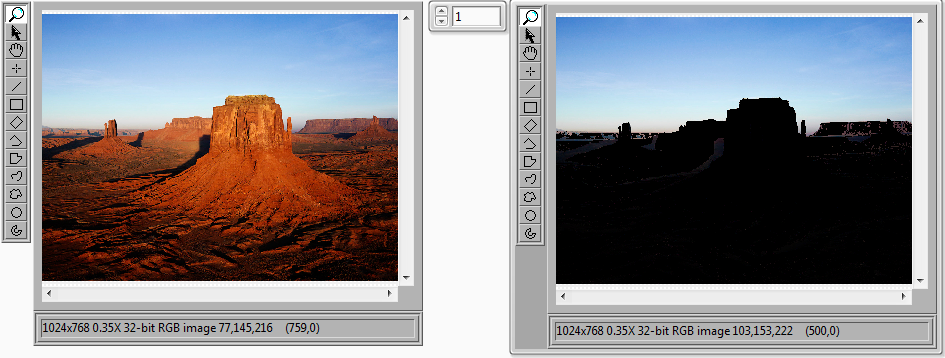
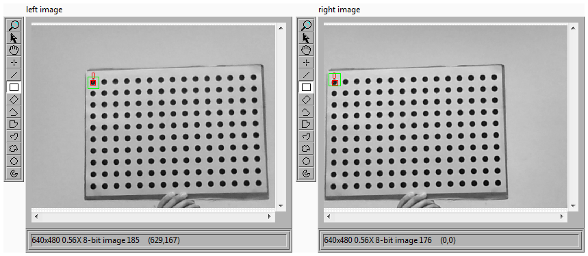
Stereo vision (OpenCV and Labview comparison)
lizhuo_lin
on:
Stereo vision (OpenCV and Labview comparison)
-
 张斌
on:
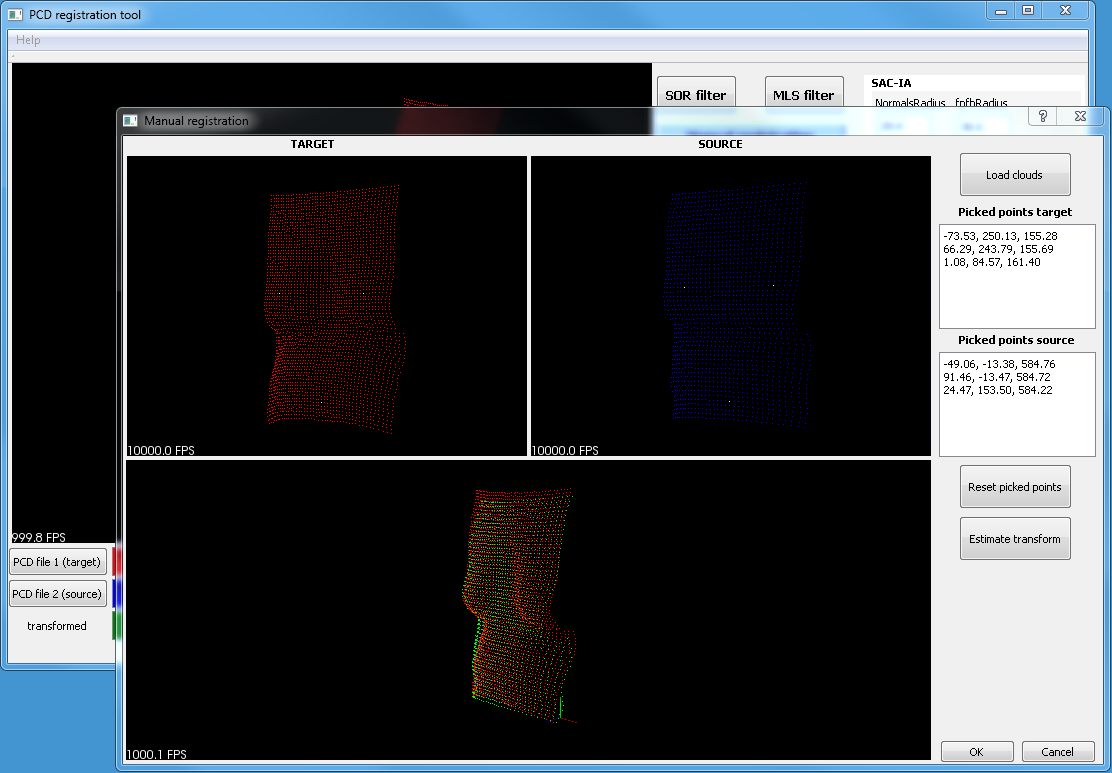
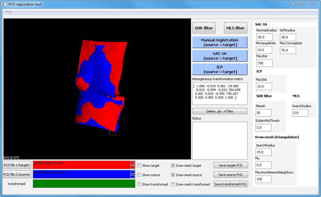
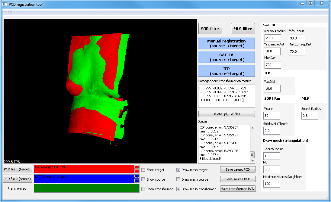
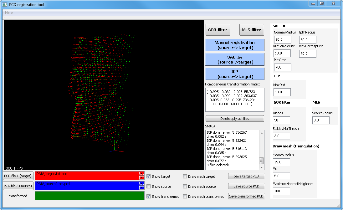
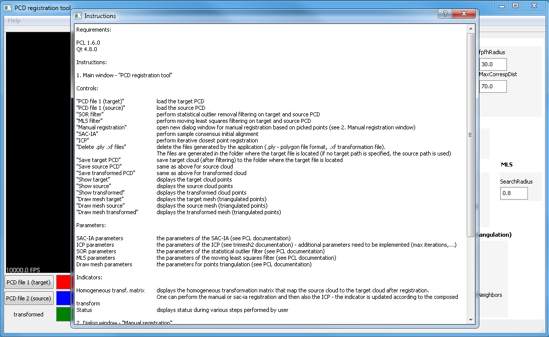
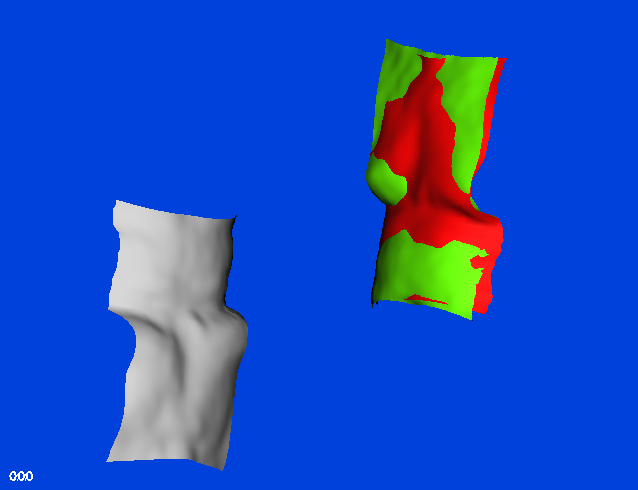
Point cloud registration tool
张斌
on:
Point cloud registration tool
-
 GohanTYO
on:
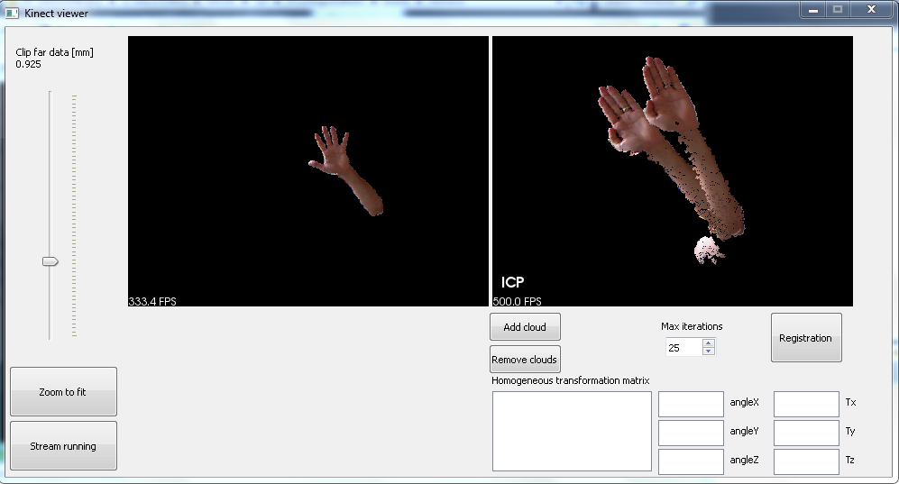
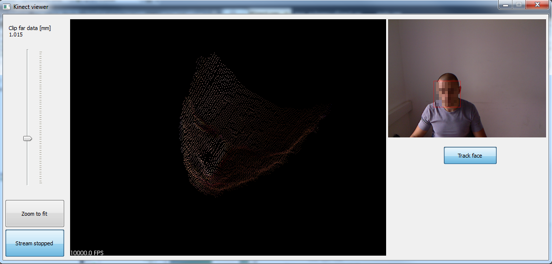
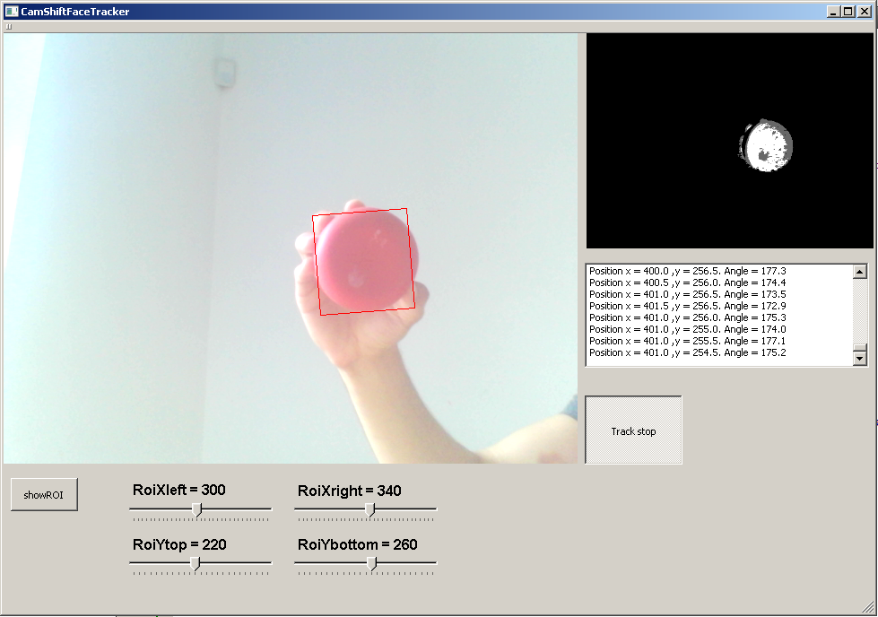
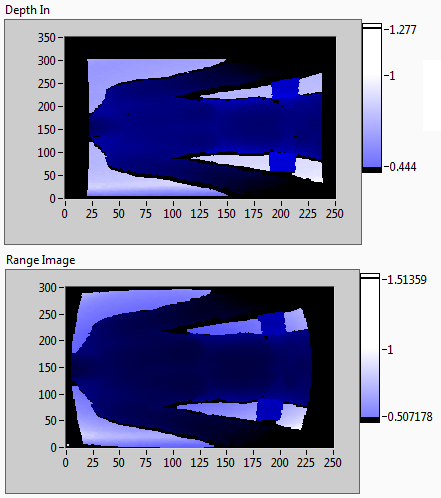
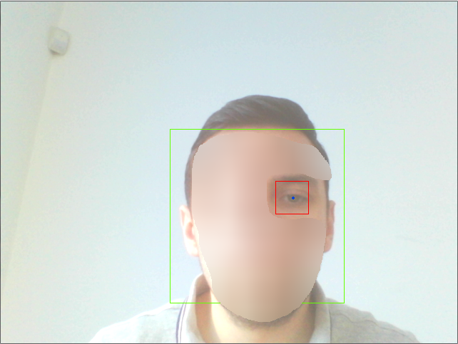
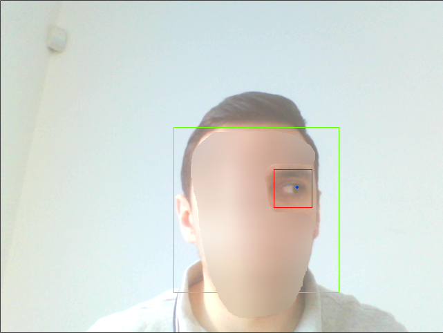
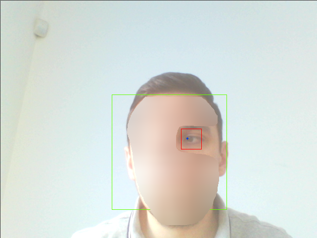
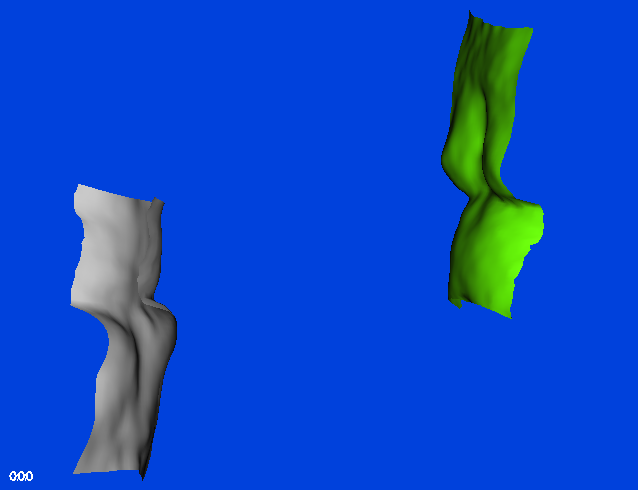
Qt+PCL+OpenCV (Kinect 3D face tracking)
GohanTYO
on:
Qt+PCL+OpenCV (Kinect 3D face tracking)
-
 Klemen
on:
Qt GUI for PCL (OpenNI) Kinect stream
Klemen
on:
Qt GUI for PCL (OpenNI) Kinect stream
-
efreet
on:
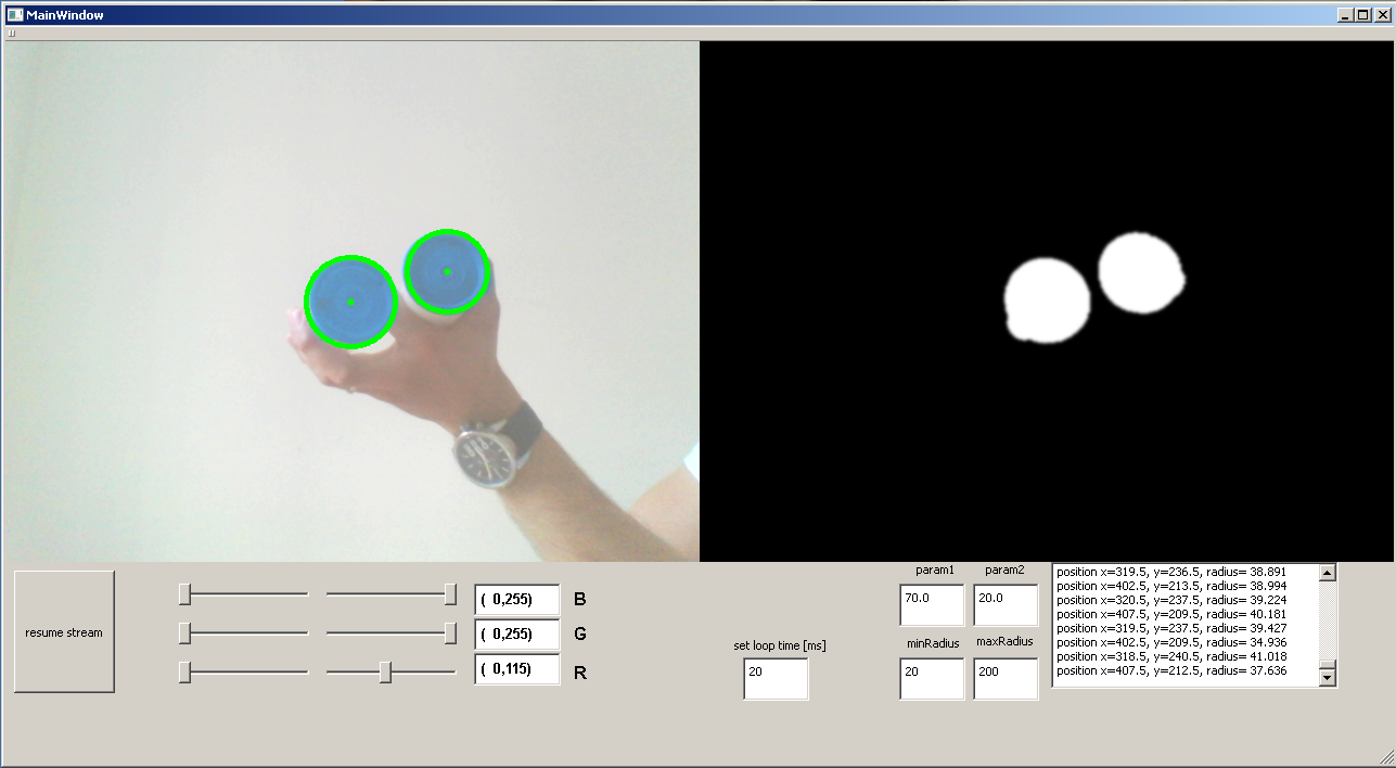
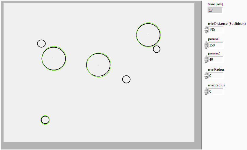
OpenCV and Qt based GUI (Hough circle detection example)
-
Spalabuser
on:
Homography mapping calculation (Labview code)
-
rameshr
on:
Optical water level measurements with automatic water refill in Labview
-
xuexue0224
on:
Kalman filter (OpenCV) and MeanShift (Labview) tracking
-
Aaatif
on:
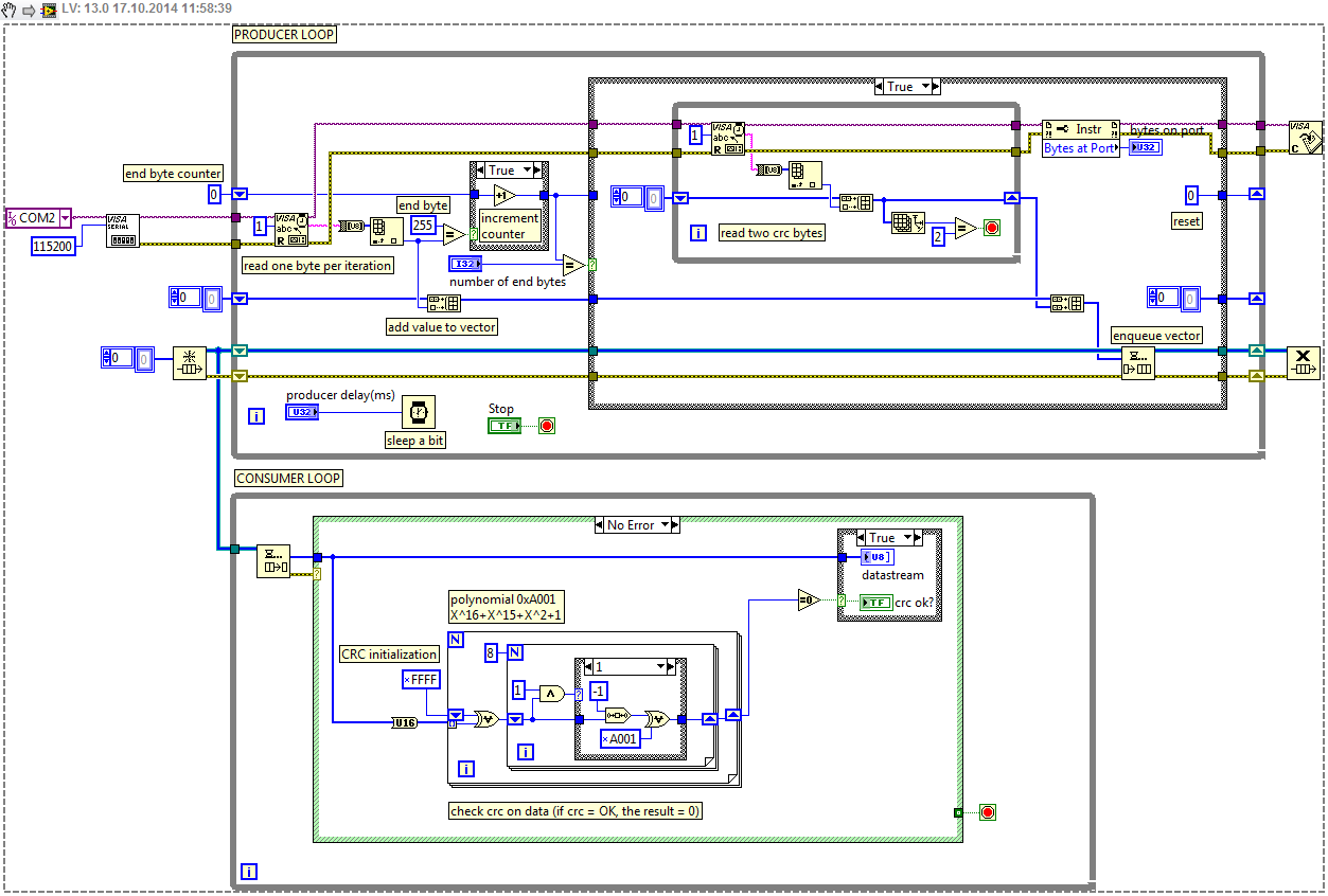
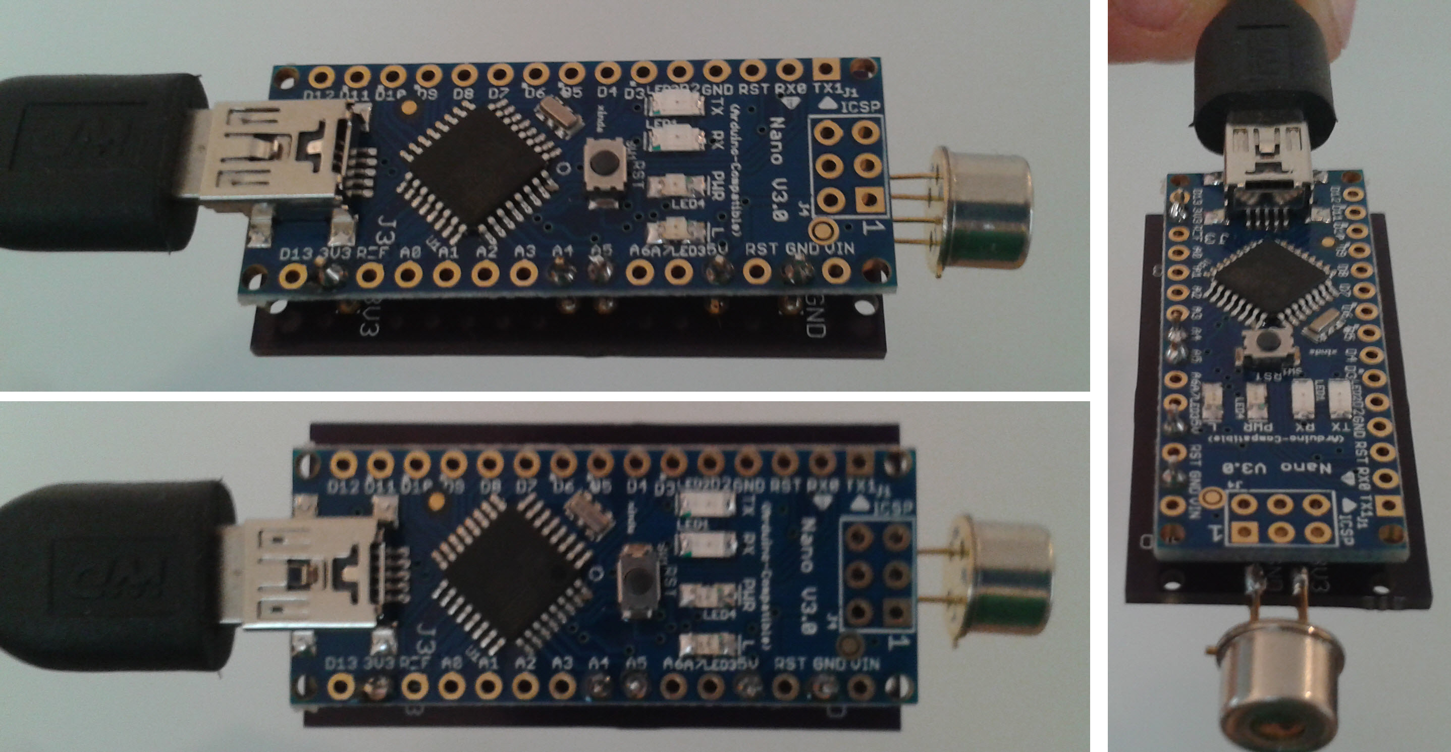
Serial data send with CRC (cyclic redundancy check) - Labview and Arduino/ARM
-
hsaid
on:
Color image segmentation based on K-means clustering using LabVIEW Machine Learning Toolkit
Turn on suggestions
Auto-suggest helps you quickly narrow down your search results by suggesting possible matches as you type.
Showing results for
Blog Options
- Mark all as New
- Mark all as Read
- Float this item to the top
- Subscribe
- Bookmark
- Subscribe to RSS Feed
11603
Views
5
Comments

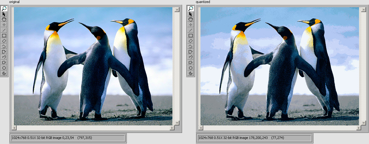
 ). There are three registration possibilities:
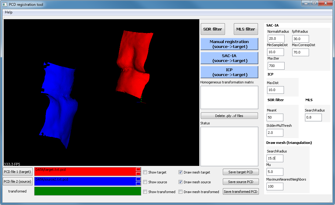
4241
Views
0
Comments

5676
Views
1
Comment
13638
Views
2
Comments
17238
Views
1
Comment
10614
Views
6
Comments


10834
Views
1
Comment


14585
Views
2
Comments
10835
Views
3
Comments


28716
Views
53
Comments
4824
Views
8
Comments

7885
Views
15
Comments

5031
Views
1
Comment

7937
Views
7
Comments
7070
Views
4
Comments
7416
Views
2
Comments

6575
Views
15
Comments
4043
Views
0
Comments
24285
Views
63
Comments
7367
Views
3
Comments
6988
Views
11
Comments
3957
Views
0
Comments
6996
Views
5
Comments

12533
Views
7
Comments
 ).
).
10483
Views
1
Comment