Community Browser
-
NI Community
- Welcome & Announcements
-
Discussion Forums
- Most Active Software Boards
- Most Active Hardware Boards
-
Additional NI Product Boards
- Academic Hardware Products (myDAQ, myRIO)
- Automotive and Embedded Networks
- DAQExpress
- DASYLab
- Digital Multimeters (DMMs) and Precision DC Sources
- Driver Development Kit (DDK)
- Dynamic Signal Acquisition
- FOUNDATION Fieldbus
- High-Speed Digitizers
- Industrial Communications
- IF-RIO
- LabVIEW Communications System Design Suite
- LabVIEW Electrical Power Toolkit
- LabVIEW Embedded
- LabVIEW for LEGO MINDSTORMS and LabVIEW for Education
- LabVIEW MathScript RT Module
- LabVIEW Web UI Builder and Data Dashboard
- MATRIXx
- Hobbyist Toolkit
- Measure
- NI Package Manager (NIPM)
- Phase Matrix Products
- RF Measurement Devices
- SignalExpress
- Signal Generators
- Switch Hardware and Software
- USRP Software Radio
- NI ELVIS
- VeriStand
- NI VideoMASTER and NI AudioMASTER
- VirtualBench
- Volume License Manager and Automated Software Installation
- VXI and VME
- Wireless Sensor Networks
- PAtools
- Special Interest Boards
- Community Documents
- Example Programs
-
User Groups
-
Local User Groups (LUGs)
- Denver - ALARM
- Bay Area LabVIEW User Group
- British Columbia LabVIEW User Group Community
- Chicago LabVIEW User Group
- Egypt NI Chapter
- GUNS
- Houston Area LabVIEW Community
- LabVIEW - University of Applied Sciences Esslingen
- [IDLE] LabVIEW User Group Stuttgart
- LUGG - LabVIEW User Group at Goddard
- LUGNuts: LabVIEW User Group for Connecticut
- Madison LabVIEW User Group Community
- Mass Compilers
- Melbourne LabVIEW User Group
- Midlands LabVIEW User Group
- Milwaukee LabVIEW Community
- Minneapolis LabVIEW User Group
- CSLUG - Central South LabVIEW User Group (UK)
- Nebraska LabVIEW User Community
- New Zealand LabVIEW Users Group
- NI UK and Ireland LabVIEW User Group
- NOCLUG
- Orange County LabVIEW Community
- Ottawa and Montréal LabVIEW User Community
- Washington Community Group
- Phoenix LabVIEW User Group (PLUG)
- Politechnika Warszawska
- PolŚl
- Rutherford Appleton Laboratory
- Sacramento Area LabVIEW User Group
- San Diego LabVIEW Users
- Sheffield LabVIEW User Group
- South East Michigan LabVIEW User Group
- Stockholm LabVIEW User Group (STHLUG)
- Southern Ontario LabVIEW User Group Community
- SoWLUG (UK)
- Space Coast Area LabVIEW User Group
- Sydney User Group
- Top of Utah LabVIEW User Group
- Utahns Using TestStand (UUT)
- UVLabVIEW
- Western NY LabVIEW User Group
- Western PA LabVIEW Users
- Orlando LabVIEW User Group
- Aberdeen LabVIEW User Group (Maryland)
- Gainesville LabVIEW User Group
- LabVIEW Team Indonesia
- Ireland LabVIEW User Group Community
- Louisville KY LabView User Group
- NWUKLUG
- LVUG Hamburg
- LabVIEW User Group Munich
- LUGE - Rhône-Alpes et plus loin
- London LabVIEW User Group
- VeriStand: Romania Team
- DutLUG - Dutch LabVIEW Usergroup
- WaFL - Salt Lake City Utah USA
- Highland Rim LabVIEW User Group
- NOBLUG - North Of Britain LabVIEW User Group
- North Oakland County LabVIEW User Group
- Oregon LabVIEW User Group
- WUELUG - Würzburg LabVIEW User Group (DE)
- LabVIEW User Group Euregio
- Silesian LabVIEW User Group (PL)
- Indian LabVIEW Users Group (IndLUG)
- West Sweden LabVIEW User Group
- Advanced LabVIEW User Group Denmark
- Automated T&M User Group Denmark
- UKTAG – UK Test Automation Group
- Budapest LabVIEW User Group (BudLUG)
- South Sweden LabVIEW User Group
- GLA Summit - For all LabVIEW and TestStand Enthusiasts!
- Bangalore LUG (BlrLUG)
- Chennai LUG (CHNLUG)
- Hyderabad LUG (HydLUG)
- LUG of Kolkata & East India (EastLUG)
- Delhi NCR (NCRLUG)
- Montreal/Quebec LabVIEW User Group Community - QLUG
- Zero Mile LUG of Nagpur (ZMLUG)
- LabVIEW LATAM
- LabVIEW User Group Berlin
- WPAFB NI User Group
- Rhein-Main Local User Group (RMLUG)
- Huntsville Alabama LabVIEW User Group
- LabVIEW Vietnam
- [IDLE] ALVIN
- [IDLE] Barcelona LabVIEW Academic User Group
- [IDLE] The Boston LabVIEW User Group Community
- [IDLE] Brazil User Group
- [IDLE] Calgary LabVIEW User Group Community
- [IDLE] CLUG : Cambridge LabVIEW User Group (UK)
- [IDLE] CLUG - Charlotte LabVIEW User Group
- [IDLE] Central Texas LabVIEW User Community
- [IDLE] Cowtown G Slingers - Fort Worth LabVIEW User Group
- [IDLE] Dallas User Group Community
- [IDLE] Grupo de Usuarios LabVIEW - Chile
- [IDLE] Indianapolis User Group
- [IDLE] Israel LabVIEW User Group
- [IDLE] LA LabVIEW User Group
- [IDLE] LabVIEW User Group Kaernten
- [IDLE] LabVIEW User Group Steiermark
- [IDLE] தமிழினி
- Academic & University Groups
-
Special Interest Groups
- Actor Framework
- Biomedical User Group
- Certified LabVIEW Architects (CLAs)
- DIY LabVIEW Crew
- LabVIEW APIs
- LabVIEW Champions
- LabVIEW Development Best Practices
- LabVIEW Web Development
- NI Labs
- NI Linux Real-Time
- NI Tools Network Developer Center
- UI Interest Group
- VI Analyzer Enthusiasts
- [Archive] Multisim Custom Simulation Analyses and Instruments
- [Archive] NI Circuit Design Community
- [Archive] NI VeriStand Add-Ons
- [Archive] Reference Design Portal
- [Archive] Volume License Agreement Community
- 3D Vision
- Continuous Integration
- G#
- GDS(Goop Development Suite)
- GPU Computing
- Hardware Developers Community - NI sbRIO & SOM
- JKI State Machine Objects
- LabVIEW Architects Forum
- LabVIEW Channel Wires
- LabVIEW Cloud Toolkits
- Linux Users
- Unit Testing Group
- Distributed Control & Automation Framework (DCAF)
- User Group Resource Center
- User Group Advisory Council
- LabVIEW FPGA Developer Center
- AR Drone Toolkit for LabVIEW - LVH
- Driver Development Kit (DDK) Programmers
- Hidden Gems in vi.lib
- myRIO Balancing Robot
- ROS for LabVIEW(TM) Software
- LabVIEW Project Providers
- Power Electronics Development Center
- LabVIEW Digest Programming Challenges
- Python and NI
- LabVIEW Automotive Ethernet
- NI Web Technology Lead User Group
- QControl Enthusiasts
- Lab Software
- User Group Lead Network
- CMC Driver Framework
- JDP Science Tools
- LabVIEW in Finance
- Nonlinear Fitting
- Git User Group
- Test System Security
- Product Groups
-
Partner Groups
- DQMH Consortium Toolkits
- DATA AHEAD toolkit support
- GCentral
- SAPHIR - Toolkits
- Advanced Plotting Toolkit
- Sound and Vibration
- Next Steps - LabVIEW RIO Evaluation Kit
- Neosoft Technologies
- Coherent Solutions Optical Modules
- BLT for LabVIEW (Build, License, Track)
- Test Systems Strategies Inc (TSSI)
- NSWC Crane LabVIEW User Group
- NAVSEA Test & Measurement User Group
-
Local User Groups (LUGs)
-
Idea Exchange
- Data Acquisition Idea Exchange
- DIAdem Idea Exchange
- LabVIEW Idea Exchange
- LabVIEW FPGA Idea Exchange
- LabVIEW Real-Time Idea Exchange
- LabWindows/CVI Idea Exchange
- Multisim and Ultiboard Idea Exchange
- NI Measurement Studio Idea Exchange
- NI Package Management Idea Exchange
- NI TestStand Idea Exchange
- PXI and Instrumentation Idea Exchange
- Vision Idea Exchange
- Additional NI Software Idea Exchange
- Blogs
-
Events & Competitions
- FIRST
- GLA Summit - For all LabVIEW and TestStand Enthusiasts!
- Events & Presentations Archive
- Optimal+
-
Regional Communities
- NI中文技术论坛
- NI台灣 技術論壇
- 한국 커뮤니티
- ディスカッションフォーラム(日本語)
- Le forum francophone
- La Comunidad en Español
- La Comunità Italiana
- Türkçe Forum
- Comunidade em Português (BR)
- Deutschsprachige Community
- المنتدى العربي
- NI Partner Hub
Latest Comments
-
 lizhuo_lin
on:
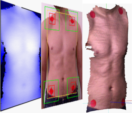
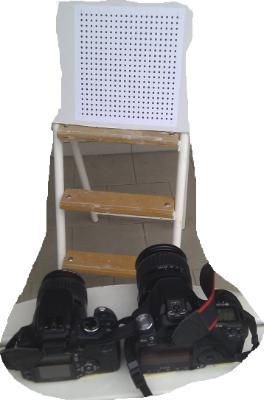
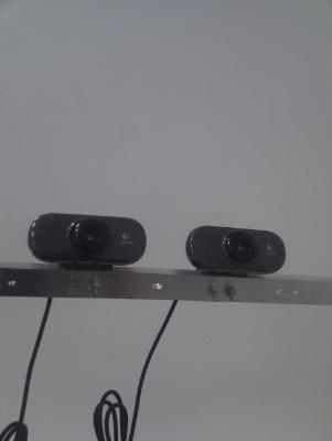
Stereo vision (OpenCV and Labview comparison)
lizhuo_lin
on:
Stereo vision (OpenCV and Labview comparison)
-
 张斌
on:
Point cloud registration tool
张斌
on:
Point cloud registration tool
-
 GohanTYO
on:
Qt+PCL+OpenCV (Kinect 3D face tracking)
GohanTYO
on:
Qt+PCL+OpenCV (Kinect 3D face tracking)
-
 Klemen
on:
Qt GUI for PCL (OpenNI) Kinect stream
Klemen
on:
Qt GUI for PCL (OpenNI) Kinect stream
-
efreet
on:
OpenCV and Qt based GUI (Hough circle detection example)
-
Spalabuser
on:
Homography mapping calculation (Labview code)
-
rameshr
on:
Optical water level measurements with automatic water refill in Labview
-
xuexue0224
on:
Kalman filter (OpenCV) and MeanShift (Labview) tracking
-
Aaatif
on:
Serial data send with CRC (cyclic redundancy check) - Labview and Arduino/ARM
-
hsaid
on:
Color image segmentation based on K-means clustering using LabVIEW Machine Learning Toolkit
Turn on suggestions
Auto-suggest helps you quickly narrow down your search results by suggesting possible matches as you type.
Showing results for
Blog Options
- Mark all as New
- Mark all as Read
- Float this item to the top
- Subscribe
- Bookmark
- Subscribe to RSS Feed
6534
Views
10
Comments
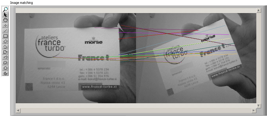
 ). The modification to use SURF algorithm is then simple. Note that the algorithm uses default parameters that cannot be altered with the attached code. But again, to extend the code to be able to change the parameters is also simple.
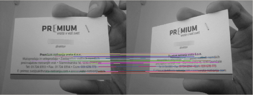


7334
Views
4
Comments


7595
Views
0
Comments

10990
Views
7
Comments

5182
Views
6
Comments
 ). The functions and VI's that are included in LabVIEW's NI Vision Module are stable, fast and most important – they perform well (sincere thanks to the developers for this). I just wish the Vision Module would by default include other popular computer vision algorithms for features detection, object tracking, segmentation, etc. (SIFT, MSER, SURF, HOG, GraphCut, GrowCut, RANSAC, Kalman filter…). Of course, one could write algorithms for achieving this, but like I said previously this is not so trivial for me, since a lot of background in mathematics and computer science is needed here. For example, Matlab has a lot of different computer vision algorithms from various developers that can be used. Since LabVIEW includes MathScript (support for .m files and custom functions) it would be interesting to try and implement some of the mentioned algorithms.