- Subscribe to RSS Feed
- Mark Topic as New
- Mark Topic as Read
- Float this Topic for Current User
- Bookmark
- Subscribe
- Mute
- Printer Friendly Page
OBJ File Format for 3D Robot Simulations
01-11-2016
08:50 PM
- last edited on
04-05-2024
02:35 PM
by
![]() Content Cleaner
Content Cleaner
- Mark as New
- Bookmark
- Subscribe
- Mute
- Subscribe to RSS Feed
- Permalink
- Report to a Moderator
Overview
Edited in July 2019 to make the attached code compatible with Haro3D 2.0 or later.
3D objects can be loaded into LabVIEW and displayed using 3D picture controls. LabVIEW natively uses a few file formats (.vrml, .dae, .stl, and .lvsg) to load 3D objects from files. A tutorial shows how to convert CAD models into LabVIEW 3D objects and use the Model Builder from the Robotic module to be able to move the robot axes. In the present document, an alternative approach that uses the OBJ file format is given.
The Wavefront OBJ file format (.obj file extension) is one of the most popular format for 3D objects with textures. Thousands of files representing almost any object can be found online. The Haro3D™ library from HaroTek (www.harotek.com) provides the ability to load those files into LabVIEW 3D picture controls. The Haro3D library is certified LabVIEW compatible and is part of the LabVIEW Tool Network.
A simple VI was developed to demonstrate how to load the .obj files corresponding to the various robot axes and how to make those axes move. No texture is used here, only the color parameters as defined in the .mtl files accompanying the .obj files.
Details on the VI are given below. This VI can be downloaded from the present document along with the robot meshes given as examples. The front panel of the VI is shown below.
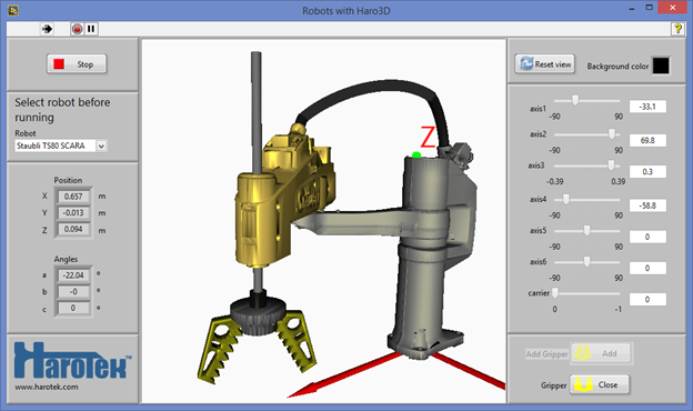
Front panel of the main VI demonstrating the use of OBJ file format for 3D robot simulations.
There are 4 robot models that are provided with the VI: 2 SCARA robots: Staubli TS80 (shown above), and Epson G20, and two articulated robots: Kuka KR120 R3900 and ABB IRB4600 (the last 3 robots are shown in the figure below). Notice that the gripper is the same for all robot models and was specifically designed by HaroTek for this demonstration.
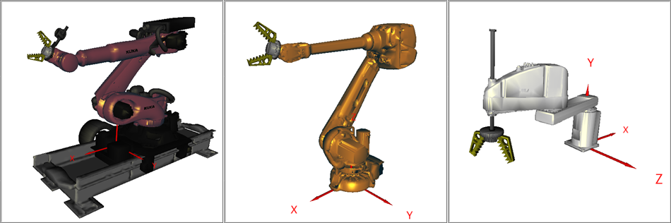
Robot models provided for demonstration. The models are from left to right: Kuka KR120 R3900, ABB IRB400, and Epson G20 (in additon of the Staubli TS80 shown in the previous figure).
The robot CAD models were obtained from the robot manufacturer websites.
The OBJ file format
The OBJ file format is a mesh file format, similar to the STL file format. The STL file format can be natively used to load 3D meshes into LabVIEW. The OBJ file format presents several advantages over the STL file format: the OBJ file format supports different types of polygons, it supports colors and textures, and mostly is extremely popular (thousands of models are available). More information about the OBJ format can be found at https://en.wikipedia.org/wiki/Wavefront_.obj_file.
OBJ files can be loaded in LabVIEW using the OBJ_File_Load.vi from the Haro3D library. The OBJ_File_Load.vi supports only triangular and quad meshes, and the LabVIEW 3D picture controls support only a small subset of the options for colors and textures supported by the OBJ format. More details about the handling of colors by the OBJ file format are given below.
Colors and textures: material (.mtl) files
The OBJ format provides great flexibility to specify the appearance of sections of a 3D object through the use of material (.mtl) files. The rest of the current section of this document is an excerpt from the Haro3D™ manual version 1.2.2 that provides details about the .mtl file format.
More information about the .mtl file can be found at http://paulbourke.net/dataformats/mtl/.
The material appearance are defined in one or more .mtl files that generally accompany an .obj file. The .mtl file is a simple text file that is loaded by the command line "mtllib file_path" in the .obj file where file_path is the full or relative path of the .mtl file. file_path can refer to a path higher than the path of the calling .obj file by the use of a double dot (../).
There are significantly fewer options available in LabVIEW to display material properties than what is available with the OBJ file format. In the specific case of the Haro3D library, the material options available from an .obj file are briefly described here.
A section of a 3D object defined in an .obj file can have properties attributed to its appearance. A specific appearance is attributed to the face definitions following the line "usemtl material_name" where material_name is a material appearance definition.
A single .obj file can use several different material definitions, and use the same material definition more than once.
Modifying the material file
The .mtl file is a simple text file. The material definitions loaded by the OBJ_File_Load.vi can be modified by directly modifying the text of the .mtl file.
The only properties of the .mtl. file that affects the appearance of a 3D object loaded by OBJ_File_Load.vi are given in the table below. All other appearance properties generally available with the OBJ format are neglected.
|
Properties |
Effect on material appearance |
Parameters |
Range |
|
Ka |
Ambient color |
R G B |
0.0 to 1.0 |
|
Kd |
Diffuse color |
R G B |
0.0 to 1.0 |
|
Ke |
Emission color |
R G B |
0.0 to 1.0 |
|
Ks |
Scattering color |
R G B |
0.0 to 1.0 |
|
Ns |
Shininess |
S |
0 to 1000 |
|
map_Kd |
texture map (selected over map_Ka and map_Ks) |
filename |
.jpg, .bmp, or .png image format |
|
map_Ka |
texture map (selected over map_Ks) |
filename |
.jpg, .bmp, or .png image format |
|
map_Ks |
texture map |
filename |
.jpg, .bmp, or .png image format |
In the specific case of OBJ_File_Load.vi, using any of the texture map property results in the same material appearance. Also, if more than one of the three texture mapping property is specified for a given object section, only one is used, map_Kd being used in priority, and map_Ka being used over map_Ks. If additional options are specified with the texture map properties after the filename, those options are ignored. If the options are specified before the filename, OBJ_File_Load.vi generates an error. It is therefore preferable to simply delete the options between the texture map property and the filename. Notice that adding the # character in front of a line of an .mtl file transforms that line into a comment ignored by OBJ_File_Load.vi. It is suggested to copy the lines before modification and to use the # character in front of the original lines to keep the full information of the original files.
Below is an example of an .mtl file. Comments about how the various properties and parameters are handled by OBJ_File_Load.vi are shown in red.
newmtl lambert2SG -> Beginning of new material definition. If used by a part of a 3D object, this part of 3D object will use "lambert2SG X" where X is the number of times that material definition is used for the current object.
illum 4 -> Ignored
Kd 0.00 0.00 0.00 -> Diffused color (R = 0.0, G = 0.0, B = 0.0)
Ka 0.00 0.20 1.00 -> Ambient color (R = 0.0, G = 0.2, B = 1.0)
Tf 1.00 1.00 1.00 -> Ignored
map_Ks Spec.png -> Ignored because a texture for map_Kd is present.
map_Kd Color01152015.jpg -> Applies texture map from file named Color01152015.jpg
bump Bump012714.jpg -bm 0.05 -> Ignored
Ni 1.00 -> Ignored
Ks 0.00 0.00 0.00 -> Specular color (R = 0.0, G = 0.0, B = 0.0)
Conversion of CAD models into .OBJ files
The robot models included with this document were selected from those of robot manufacturers that make their CAD models readily available on their websites. The robot CAD models should be available from all manufacturers but in some cases, the CAD models can only be obtained by directly contacting the manufacturers.
The robot CAD models from the manufacturers can be in various formats but should include a generic format like IGES or STEP. The CAD model files must be converted into mesh file format like .ply, .stl, or .obj. This conversion can be done by most CAD software like Solidworks from Dassault Systèmes, Pro/Engineer from PTC, or Rhino 3D from Robert McNeel & Associates, to name a few. In the present case, the CAD models from the robot manufacturers were converted using the free open-source application FreeCAD (http://www.freecadweb.org/).
FreeCAD was used to read the original CAD files and export the axis components into mesh files. The components in the CAD files were separated by robot axes, and within each axis, by component having the same appearances (arms, name plates, harness, etc.; see figure below). All the components related to a given axis are saved in a single directory. The axis directory name becomes the name of the axis in LabVIEW and the shortest name in the directory becomes the main component of the axis. The directories for all axes must be in the same robot directory, and the directory names must be in alphabetical order of their axis hierarchy. Example of directory names are: abase, axis1, axis2, axis3, etc.

Organization of the CAD objects by axis group within FreeCAD.
The components of each axis are saved into STL format files. These files are loaded into the free open-source application Meshlab (http://meshlab.sourceforge.net/). Meshlab is used to reduce the file sizes and to correct the mesh normals. The number of faces in each file was decreased by 70% to 90% (percentage reduction in the dialog below between 0.3 and 0.1) using the Meshlab function Filters -> Remeshing, Simplification and Reconstruction -> Quadric Edge Collapse Decimation to reduce the mesh file sizes (see figure below). This reduction (and corresponding loss of visual definition) is not necessary if disk space is not an issue. File size also impacts load time into LabVIEW. The normals were calculated using the Meshlab function Filters -> Normals, Curvatures, and Orientation -> Compute Vertex Normals (Notice that Haro3D version 1.2.0 does not normalize the normal but the next version will).
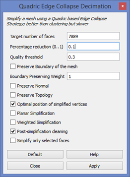
The option window of the Quadric Edge Collapse Decimation of Meshlab to reduce the number of faces in a mesh.
Each component is then exported as an .obj file. In the export options dialog the Normal box must be checked but the color boxes should be unchecked.
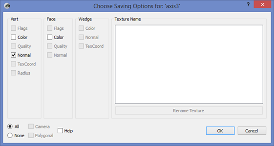
The option window of the .obj export function of Meshlab.
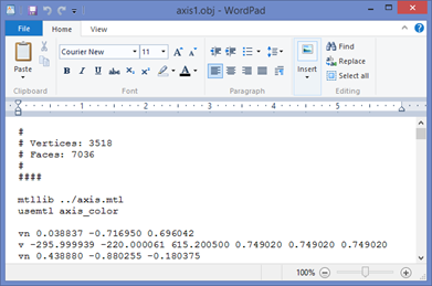
Each .obj file must then be modified using a text editor like Notepad or Wordpad to include the command line “mtllib file_path” where file_path is the path of the .mtl file containing the material definition of the current object as shown below. Notice that if any of the Color boxes had been left checked in the option dialog when exporting from Meshlab, “mtllib” and “usemtl” command lines are present and must be modified or deleted.
To provide a consistent coloring of the robot, the same .mtl files are used for all axes. For example, the main arm of an axis is colored using the axis_color properties in the axis.mtl file located in the main directory of the Kuka robot, as shown in the example below for axis1. The same commands are used for all the axis arms of the Kuka robot.
Example of calls to load a material file and use of a material definition
The file axis.mtl defines axis_color as shown in the figure below. The Kd parameter gives the robot its orange look and the Ks parameter gives it the yellowish reflection. The Ns value (500 out of a maximum of 1000) gives the robot a somewhat shiny look.

Example of appearance definition in a .mtl file
All .obj file defining the axis arms of the Kuka robot calls the same axis.mtl file that defines axis_color. The appearance of all axis arms can then be changed by modifying a single file. The other components of the axes share other .mtl files, like black_metal.mtl, black_plastic.mtl, and gray_metal.mtl, as required by the desired appearance. Note that a single .mtl file containing all material definitions could have been used as well.
VI Description
Object-Oriented Programming was used to demonstrate the concept described in this document. The code includes a single VI, Robots_with_3D_OBJ.vi and two classes: 3D_Robot and Robot_Section.
Directory structure and data files
The directory structures of the robot models are located in a directory named Models that must be located in the same directory than Robots_with_3D_OBJ.vi. In addition of the .obj files, each robot model must include moves.txt and offsets.txt files. The moves.txt file contains the type of movement associated with each axis. Each line of moves.txt gives the type of movement of an axis. The order of the text line indicates to which axis it corresponds, according to the alphabetical order of the axes. The possible values for each line are: None, Rot X, Rot Y, Rot Z, Rot Other, Trans X, Trans Y, Trans Z, Trans Other. Those values correspond to the items of the enum control arm_rot_axis.ctl. The Rot X, Y, Z values indicate that the axis rotates around an axis parallel with the X, Y, Z directions, respectively; and the Trans X, Y, Z values indicate that the axis moves along an axis parallel with the X, Y, Z directions. The Rot Other and Trans Other have not been implemented in the provided code.

Example of axis directory structure for a given robot.
The offsets.txt file contains the position offsets of the reference points of each axis. The reference point is the center of rotation for a rotating axis for example. As for the moves.txt file, the text line order corresponds to the alphabetical order of the axes. The moves.txt and offsets.txt files provide the information required to appropriately move each robot axis, and to correctly calculate the forward kinematics.
All the .obj files that are part of a single axis must be in a single directory. The axis name will be the name of the directory. The directories must be named in alphabetical orders of their order on the robot. For example, the robot base directory must be renamed “abase” so that its alphabetical order precedes “axis1”. In the figure above, the rail directory is named “aaarail”, the carrier is renamed “aacarrier”, and the robot base is named “abase”, indicating the hierarchy of the components. In each directory, the file with the shortest names is the reference object for that axis (see figure below).
The offsets are the values relative to the previous axis. For example, offset of axis3 is the position of the reference point of axis3 relative to the position of the reference point of axis2. The offsets can generally be extracted from the specification documents provided by the robot manufacturers. If the offsets are not available from documents, they can be measured from the CAD model. The offset of the first axis (either the base or rail) is relative to the origin in the CAD model.
The orientation of the translation or rotation depends on the orientation of the CAD model.

Example of files within one axis directory.
The meshes included with this document includes a gripper to demonstrate how to attach a tool at the end of each robot. The tool was designed separately from the robots and has its own origin, different from those of the robot models. Its main axis is orientated parallel with the X direction. The tool need to be reoriented if the X-axis orientation is not adequate for a given robot. If a tool is included and properly positioned in the CAD model of a robot, the tool .obj files can simply be treated as another axes of the robot.
Code
The provided code consists of a single VI, Robots_with_3D_OBJ.vi, and of two classes, 3D_Robot and Robot_Section. The VI calls the Init method of the 3D_Robot class that creates an array of Robot_Section objects corresponding to each of the directory of the provided path corresponding to the selected robot (see figure below).

Initialization of the 3D_Robot object.
When an axis control value is changed, the caption text of the control is used to identify the axis that is being moved. The captions of each axis control was given the name of its corresponding axis directory (aacarrier for the carrier control for example). The use of the captions here instead of the labels prevents from having awkward identification of the controls on the front panel.
The value is passed to the Move_Axis method along with the index of the axis moved. The axis is moved in the 3D picture control using the 3D object reference within the corresponding Robot_Section object.
The values of all the controls are passed to the Forward_Kinematics method to calculate the position and angles of the end of the robot, either the last axis or the tool, if the latter had been added. A value must be provided for all axes, even for those that do not have movement associated with them.
The number of control values is also limited to the number of axes of the current robot.
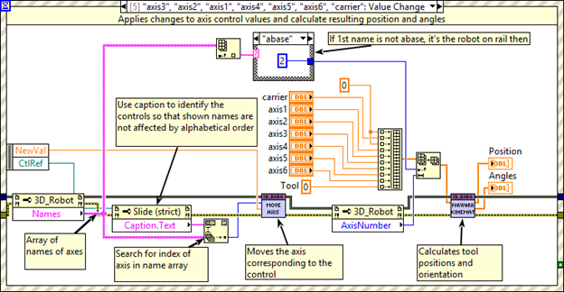
Handling of the axis movements and of the kinematics calculation using the Move_Axis and Forward_Kinematics methods.
The tool is added by clicking the “Add gripper” button. The tool is added by using the Load_Tool method. The offset provided is going to be used by the Forward_Kinematics method to calculate the desired position. Notice that the tool needs to be rotated, depending on the robot used. The last axis of the SCARA robots does not have the same orientation than the last axis of an articulated robot. In addition, the Epson CAD model does not have the same orientation than the other robot CAD models.
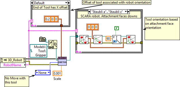
Addition of a tool using the Load_Tool method and orientation adjustment according to the selected robot.
The tool can be opened and closed using the “Gripper” button. The operation of the tool is provided as an example but is not generic and would depend on each specific tool.
The CleanUp method is called to release the references before exiting the VI.
Requirements
The attached VI requires Haro3D library version 1.2.0. The Haro3D library can be downloaded using VIPM.
The attached VI and classes are compatible with LabVIEW 2013 or later.
Installation
Just unzip the attached file in a given directory.
Operations of the VI
The desired robot must be selected from the drop-down menu before running the VI.
Just open Robots_with_3D_OBJ.vi, select the desired robot and run the VI.
The controls can control rotations or translations, depending on the specific axis of each robot. The angle units are degrees, and the translation units are in meters. Notice that for the robots that do not have the corresponding axes (like axis5, axis6 and carrier for the SCARA robots), changing the values of those controls generates an error and terminates the VI. Also, the limits on the axis controls must be manually set if desired.
Clicking the “Add gripper” button adds a tool at the end of the last axis of the current robot. The “Gripper” button becomes enabled. Clicking the “Gripper” button opens and closes the tool.
The VI is stopped by clicking the close window box or the stop button.
Summary
This document shows how to use the OBJ file format to load a robot from its CAD model into a LabVIEW 3D picture control. The use of the OBJ file format requires the Haro3D library. The attached VI and classes can be modified to use the same approach with STL format files but the appearance of the objects will have to be handled from within the code.
The OBJ file format supports texture but no texture is used in this document. The use of textures with the OBJ format will be discussed in a separate document.
Do not hesitate to edit the material files to experiment on the appearance of the robots. The correct parameters can be tricky to determine but the results can be interesting.
If you have any question concerning this document or the utilization of the VI, or if you have a robot CAD model that is publicly available that you want converted, do not hesitate to contact me.
